![Exhibit: Linear functional relation - Fahrenheit by Celsius degrees conversion [m15005.jpg]](m15005.jpg)
![Exhibit: Curvilinear functional relation - BMI by height for constant weight (70 kg) [m15004.jpg]](m15004.jpg)
![Exhibit: A linear statistical relation - female by male life expectancy [m15002.jpg]](m15002.jpg)
![Exhibit: A curvilinear statistical relation - female life expectancy by doctors per million [m15003.jpg]](m15003.jpg)
![Exhibit: Pictorial representation of simple linear regression model (NWW figure 18.4 p. 535) [m15006.gif]](m15006.gif)
![Exhibit: Simple linear regression of % clerks (Y) on seasonality (X) [m15001.jpg]](m15001.jpg)
![Exhibit: Regression of % clerks on seasonality showing the meanings of b0 and b1 [m15008.gif]](m15008.gif)
![Exhibit: Vertical deviations ei of Yi from regression line involved in estimating b0 and b1 by OLS [m15010.gif]](m15010.gif)
A statistical relation between a dependent variable
Y and an independent variable X is an inexact relation; the value of Y
is not uniquely determined when the value of X is specified.
"line or curve of statistical relationship" = tendency of Y to vary systematically as a function of X
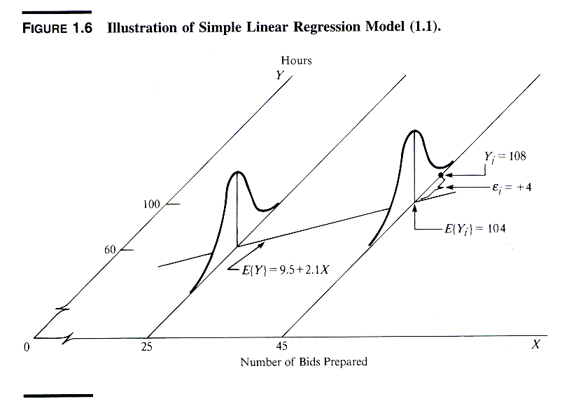
Exhibit: Pictorial representation of simple linear regression model (NWW figure 18.4 p. 535) [m15006.gif] Exhibit: Pictorial representation of simple linear regression model (NKNW F1.6 p. 12)
Yi = b0 + b1Xi + ei i = 1, 2, ..., nwhere
Yi is the value of the dependent variable for the ith observation
Xi is the value of the independent (predictor) variable for the ith element, and is assumed to be a known constant
b0 and b1 are parameters (or coefficients)
ei are independent ~N(0,s2)
E{Y} = b0 + b1X
From the simple linear regression model
E{Yi} = E{b0 + b1Xi + ei} = b0 + b1Xi + E{ei}Since E{ei} = 0 it follows that E{Yi} = b0 + b1Xior, in general for any value of X E{Y} = b0 + b1X |
The graph of the regression function is called
the regression line.
The parameters b0
and b1X
are called regression coefficients or regression parameters.
The meaning of each coefficient is as follows
Q - What is the meaning of the slope (-.169) in the regression of % clerks on the seasonality index?Exhibit: Regression of % clerks on seasonality showing the meanings of b0 and b1 [m15008.gif]
s2{Yi} = s2{b0 + b1Xi + ei} = s2{ei} = s2since ei is the only RV in the expression, and the variance of the eror ei is assumed the same (= s2 ) regardless of the value of X.
Q = Si=1 to n (Yi - b0 - b1Xi)2The following exhibit shows the Y (vertical) deviations ei that are squared and summed up to evaluate Q (although in this case the regression line is already the OLS solution) Q can be minimized by:
b1 = (S(Xi - X.)(Yi - Y.))/S(Xi - X.)2(calculating b1 first, then b0)
b0 = Y. - b1X.
Q - What is the meaning of these formulas?
To find the values of b0
and b1
that minimize
Q = Si=1 to n (Yi - b0 - b1Xi)2one differentiates Q with respect to b0 and b1, obtaining dQ/db0 = -2Si=1 to n (Yi - b0 - b1Xi)The particular values, denoted b0 and b1, that minimize Q are found by setting these derivatives to zero, as -2Si=1 to n (Yi - b0 - b1Xi) = 0and solving for b0 and b1. Solving is done by simplifying and expanding these equations and rearranging the terms to produce the normal equations SYi = nb0 + b1SXipresented earlier. |
Table 1 shows how the regression coefficients can be calculated using
these formulas for the Stinchcombe data (elements are sectors of the construction
industry, Yi is % clerks, and Xi is an index of seasonality
of employment).
|
|
Sector | Xi | Yi | (Xi - X.) | (Yi - Y.) | (Xi - X.)2 | (Yi - Y.)2 | (Xi - X.)
x (Yi - Y.) |
| 1 | STRSEW | 73 | 4.8 | 33.444 | -3.156 | 1118.531 | 9.958 | -105.536 |
| 2 | SAND | 43 | 7.6 | 3.444 | -0.356 | 11.864 | 0.126 | -1.225 |
| 3 | VENT | 29 | 11.7 | -10.556 | 3.744 | 111.420 | 14.021 | -39.525 |
| 4 | BRICK | 47 | 3.3 | 7.444 | -4.656 | 55.420 | 21.674 | -34.658 |
| 5 | GENCON | 43 | 5.2 | 3.444 | -2.756 | 11.864 | 7.593 | -9.491 |
| 6 | SHEET | 29 | 11.7 | -10.556 | 3.744 | 111.420 | 14.021 | -39.525 |
| 7 | PLUMB | 20 | 10.9 | -19.556 | 2.944 | 382.420 | 8.670 | -57.580 |
| 8 | ELEC | 13 | 12.5 | -26.556 | 4.544 | 705.198 | 20.652 | -120.680 |
| 9 | PAINT | 59 | 3.9 | 19.444 | -4.056 | 378.086 | 16.448 | -78.858 |
| Total | 356 | 71.6 | -0.000 | 0.000 | 2886.222 | 113.162 | -487.078 | |
| Mean | 39.556 | 7.956 |
b0 and b1 are then calculated using the formulas above as
b1 = (-487.078)/(2886.222) = -0.169(The slope b1 can also be calculated as the ratio of the same two numbers, each divided by n-1, i.e. as the sample covariance of X and Y, denoted sXY, divided by the variance of X, denoted sX2, as
b0 = (7.956) - (-0.169)(39.556) = 14.631
b1 = sXY/sX2
b0 = Y. - b1X. )
^Y = b0 + b1Xwhere ^Y ("Y hat") is the estimated regression function at level X of the independent variable.
^Y = 14.631 - (0.169)X is the estimated regression function
^Y8 = 14.631 - (0.169)(13) = 12.437 is the fitted value for observation 8 (ELEC)
E{Yh} = b0 + b1Xhwhere Xh denotes a specified level of X that does not necessarily correspond to the value Xi of an observation in the sample.
^Yh = b0 + b1XhExample: if a sector of the construction industry had a seasonality score Xh = 35 (a value not found in the data set), the estimated mean response would be
^Yh = 14.631 - (0.169)(35) = 8.716
ei = Yi - ^Yiso ei corresponds to the vertical discrepancy between Yi and the corresponding point ^Yi on the regression line.
|
|
|
|
|
|
|
|
|
|
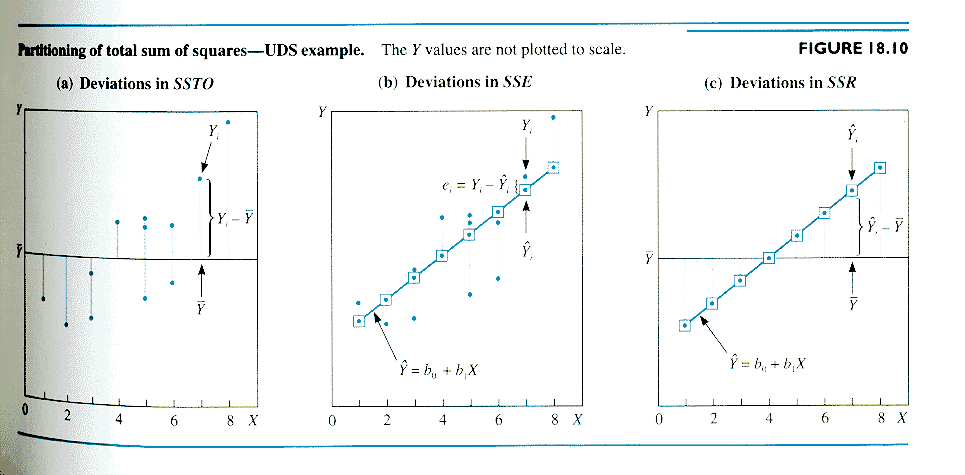
One defines sums of squares corresponding to
each deviation:
| Symbol |
|
|
|
| Formula |
|
|
|
| Name |
|
|
|
| Meaning |
|
|
|
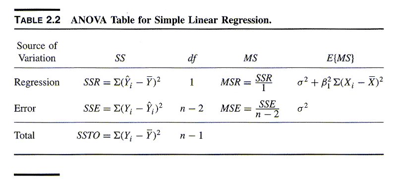
The basic ANOVA result is:
|
|
|
|
|
|
|
|
|
|
|
|
|
|
This is actually a remarkable and non-obvious
property that must be proven! (See optional proof in NWW p. 552 (bottom).)
Table 2 shows the calculations of ANOVA sums
of squares for the regression of % clerks (Y) on employment seasonality
(X).
|
|
|
|
|
|
|
(Yi - Y.)2 | (^Yi - Y.)2 | (Yi - ^Yi)2 |
| 1 | STRSEW | 73 | 4.8 | 2.311 | 2.489 | 9.958 | 31.856 | 6.193 |
| 2 | SAND | 43 | 7.6 | 7.374 | 0.226 | 0.126 | 0.338 | 0.051 |
| 3 | VENT | 29 | 11.7 | 9.737 | 1.963 | 14.021 | 3.173 | 3.854 |
| 4 | BRICK | 47 | 3.3 | 6.699 | -3.399 | 21.674 | 1.578 | 11.555 |
| 5 | GENCON | 43 | 5.2 | 7.374 | -2.174 | 7.593 | 0.338 | 4.727 |
| 6 | SHEET | 29 | 11.7 | 9.737 | 1.963 | 14.021 | 3.173 | 3.854 |
| 7 | PLUMB | 20 | 10.9 | 11.256 | -0.356 | 8.670 | 10.891 | 0.127 |
| 8 | ELEC | 13 | 12.5 | 12.437 | 0.063 | 20.652 | 20.084 | 0.004 |
| 9 | PAINT | 59 | 3.9 | 4.674 | -0.774 | 16.448 | 10.768 | 0.599 |
| Total | 356 | 71.6 | 113.162 | 82.199 | 30.963 | |||
| Mean | 39.556 | 7.956 |
|
|
|
|||
| b1 = | -0.169 | |||||||
| b0 = | 14.631 |
Alternative computational formulas are:
|
|
|
|
|
|
|
|
|
|
||
|
(cf. sample variance s2) |
|
b0 and b1 |
|
|
|
|
|
|
|
|
|
|
|
|
MSE is an estimator of s2,
the variance of e.
(This makes sense since MSE is the sum of
the squared residuals divided by the df of this sum, which is n-2.)
It can be shown that MSE is an unbiased estimator
of s2,
i.e.
E{MSE} = s2(MSE)1/2, called the standard error of estimate, is an estimator of s, the standard deviation of e.
| Source | Sum of Squares | df | Mean Squares | F-ratio |
| Regression | 82.199 | 1 | 82.199 | 18.583 |
| Error | 30.963 | 7 | 4.423 | |
| Total | 113.162 | 8 | 14.145 |
The F-ratio is calculated as the ratio F* = MSR/MSE (here 82.199/4.423 = 18.583); the meaning of F* is discussed in Module 16.
Q - What are the meanings of the quantities 4.423 and 14.145 in Table 3?
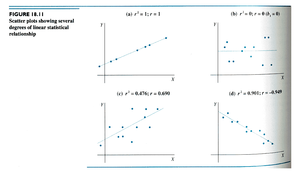
r2 = (SSTO - SSE)/SSTO = SSR/SSTO = 1 - SSE/SSTOwhere 0 <= r2 <= 1
Example: In the regression of % clerks on seasonality the r2 can be calculated equivalently as
(113.162 - 30.963)/113.162 = 82.199/113.162 = 1 - (30.963/113.162) = 0.726Limiting cases:
r = +/- (r2)1/2 = (S(Xi - X.)(Yi - Y.))/(S(Xi - X.)2S(Yi - Y.)2)1/2The "+/-" means that r takes the sign of b1.
|r| > r2so that the psychological impact (or propaganda value) of r is stronger than that of r2.
b1* = b1(sX/sY)which in the simple linear regression model is equal to r. (This is no longer true in the multiple regression model.)
b1 = b1*(sY/sX) ( = r(sY/sX), in simple linear regression only)where sX and sY are the sample standard deviations of X and Y, respectively.
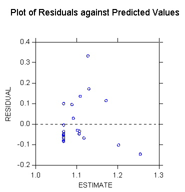
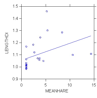
>rem relationship
berween sex dimorphism (length ration male to female) and
>rem mean harem size
in primates, a measure of sexual competition among males
>regress
>model lengthdi=constant+meanhare
>estimate
Dep Var: LENGTHDI N: 22 Multiple R: 0.403 Squared multiple R: 0.162
Adjusted squared multiple R: 0.120 Standard error of estimate: 0.115
Effect
Coefficient Std Error Std Coef
Tolerance t P(2 Tail)
CONSTANT
1.055 0.035
0.000 . 29.949
0.000
MEANHARE
0.014 0.007
0.403 1.000 1.967
0.063
Analysis of Variance
Source
Sum-of-Squares df Mean-Square
F-ratio P
Regression
0.051 1
0.051 3.870
0.063
Residual
0.266 20 0.013
-------------------------------------------------------------------------------
*** WARNING ***
Case
17 has large leverage (Leverage =
0.487)
Case
19 is an outlier (Studentized
Residual = 3.821)
Durbin-Watson D Statistic
1.949
First Order Autocorrelation
-0.026
>plot lengthdi*meanhare/stick=out smooth=linear short
>USE "Z:\mydocs\ys209\yule.syd"
SYSTAT Rectangular file
Z:\mydocs\ys209\yule.syd,
created Wed Feb 17,
1999 at 09:34:32, contains variables:
UNION$
PAUP OUTRATIO
PROPOLD POP
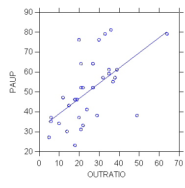
>model paup=constant+outratio
>estimate
Dep Var: PAUP
N: 32 Multiple R: 0.594 Squared multiple R: 0.353
Adjusted squared multiple
R: 0.331 Standard error of estimate: 13.483
Effect
Coefficient Std Error Std Coef
Tolerance t P(2 Tail)
CONSTANT
31.089 5.324
0.000 .
5.840 0.000
OUTRATIO
0.765 0.189
0.594 1.000 4.045
0.000
Analysis of Variance
Source
Sum-of-Squares df Mean-Square
F-ratio P
Regression
2973.751 1 2973.751
16.359 0.000
Residual
5453.468 30 181.782
-------------------------------------------------------------------------------
*** WARNING ***
Case
15 has large leverage (Leverage =
0.328)
Durbin-Watson D Statistic
1.853
First Order Autocorrelation
-0.018
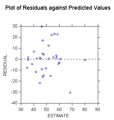
>plot paup*outratio/stick=out smooth=linear short
. use "Z:\mydocs\S208\gss98.dta", clear
. su income
Variable
| Obs
Mean Std. Dev. Min
Max
-------------+-----------------------------------------------------
income | 2699 10.85624
2.429604 1
13
. su educ
Variable
| Obs
Mean Std. Dev. Min
Max
-------------+-----------------------------------------------------
educ | 2820 13.25071 2.927512
0 20
. regress income educ
Source | SS
df MS
Number of obs = 2688
-------------+------------------------------
F( 1, 2686) = 235.66
Model | 1269.91329 1 1269.91329
Prob > F = 0.0000
Residual
| 14474.0495 2686 5.38870049
R-squared = 0.0807
-------------+------------------------------
Adj R-squared = 0.0803
Total | 15743.9628 2687 5.85930882
Root MSE = 2.3214
------------------------------------------------------------------------------
income | Coef. Std. Err.
t P>|t| [95% Conf. Interval]
-------------+----------------------------------------------------------------
educ | .2359977 .0153731 15.35
0.000 .2058533 .2661421
_cons | 7.71967 .2094621
36.85 0.000 7.308947
8.130393
------------------------------------------------------------------------------