soci209 - module 11 - collinearity diagnostics & remedies

Module 11 - COLLINEARITY

(Sometimes "multicollinearity". Belsley, Kuh, and Welsch (1980) dislike "multi-" as redundant.)

1. SYMPTOMS OF COLLINEARITY

The following symptoms may indicate a collinearity problem

large changes in b_k when adding or deleting variables(s) or observation(s)
b_k non significant for a theoretically important X_k
b_k with sign opposite of expected (from theory or previous results)
large correlations(s) in r_XX
wide s{b_k} for important X_k(s)
b_ks are non significant even though F for whole regression is significant

Note in the next exhibits how correlations among independent variables are not extreme, as seen in the splom, but in the regression regression coefficients are n.s. despite high R².

2. TOLERANCE (TOL) & VARIANCE INFLATION FACTOR (VIF)

The tolerance for variable X_k is

(TOL)_k = 1 - R_k² k = 1, 2, ..., p-1

where R_k² is the R square when X_k is regressed on the other independent variables in the model including a constant.
The variance inflation factor for variable X_k is the inverse of the tolerance

(VIF)_k = 1/(TOL)_k

Why the expression "variance inflation factor"?

The standardized regression model is a regression model in which all the variables (X and Y) are standardized into z-scores with mean 0 and standard deviation 1, and divided by (n - 1)^1/2 (see NKNW Section 7.5, pp. 277-284).
In the standardized regression model the normal equations X'Xb = X'Y become

r_XXb* = r_YX

where r_XX is the matrix of correlations of X, r_YX are the correlations of Y with the X, and b* is the vector of standardized regression coefficients.
One can show that (VIF)_k is the kth diagonal element of (r_XX)^-1 so that

s²{b_k*} = (s*)²(VIF)_k = (s*)²/(1 - R_k²)

where (s*)² is the error variance of the standardized model.
Thus (VIF)_k measures how much the variance of the standardized regression coefficient b_k* is inflated by collinearity.

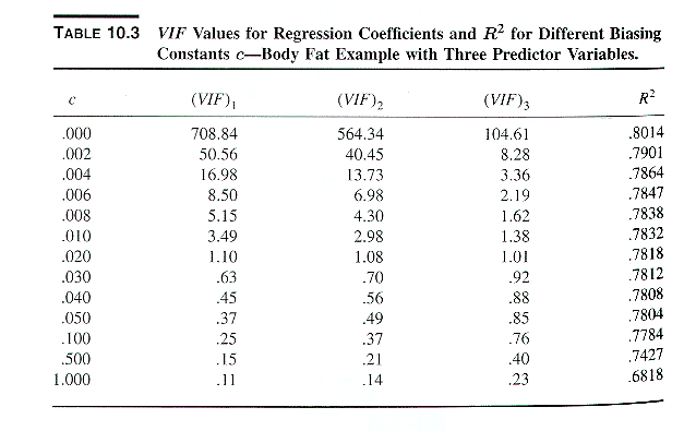
Using TOL or VIF for Diagnosis

As discussed earlier, a common rule of thumb is to take

TOL < .1 or equivalently
VIF > 10

as an indication that collinearity may be a problem.
For the body fat data the values of TOL andVIF) are

Independent variable	TOL	VIF
TRICEPS	.001411	708.717
THIGH	.001772	564.334
MIDARM	.00956	104.603

These values indicate high collinearity levels.
Similarly, the average VIF

(VIF). = (S_{i=1
to p-1} (VIF)_k)/(p-1)

is an indicator of collinearity for the entire model.

3. (Optional) ADVANCED COLLINEARITY DIAGNOSTICS

Advanced collinearity diagnostics discussed by Belsley, Kuh, and Welsh (1980) are output by SYSTAT with the extended output option (print = long). The following exhibits show advanced diagnostics for the body fat data and for the Longley data:

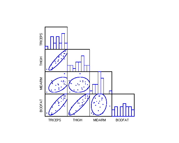
The following diagnostics are produced (see body fat exhibit):

factorization of the correlation matrix r_XX into its eigenvalues and eigenvectors (long story omitted, available upon request); many eigenvalues close to 0 suggest that the variables are redundant (i.e., collinear); for the body fat data the second eigenvalue is already only .021, indicating high redundancy
the condition indices (CI) are the square roots of the ratios of the largest eigenvalue to each successive eigenvalue; according to Kuh, Belsley, and Welsh (1980) CI > 15 indicates a possible problem, and CI > 30 a serious problem with collinearity; the last (largest) CI is called the condition number of the r_XX matrix; a matrix with a high condition number is called ill-conditioned; in the body fat data the 3d index is 18.566 and the 4th is a whopping 677.372
the variance proportions are the proportions of the variance of the estimates accounted for by each eigenvector (also called principal component) associated with each of the eigenvalues; "You should begin to worry about collinearity when a component associated with a high condition index contributes substantially to the variance of two or more variables." (SYSTAT Statistics V6.0/V7.0 p. 265); in the body fat data the 4th principal component "loads" heavily on all three independent variables (.998, 1.000, .992) indicating a severe collinearity problem
large absolute values in the correlation matrix of regression coefficients also suggest collinearity; in the body fat data the three intercorrelations of the independent variables (-.999, -.995, .994) are very high in absolute value, confirming the collinearity problem

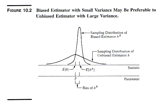
These diagnostics are further explained in Belsley, Kuh, and Welsh (1980). In my experience with a number of data sets these advanced diagnostics are sometimes inconclusive; a common pattern is conclusion of high collinearity involving the constant term, or another variable, when in fact there is no collinearity problem with that variable. In most cases TOL or VIF is a sufficient diagnostic of collinearity.

4. REMEDIES FOR COLLINEARITY

The fundamental problem with collinearity is that the pattern of intercorrelations among variables makes the X'X matrix nearly singular, which makes estimation of the regression coefficients imprecise/unstable. Once collinearity has been diagnosed, a number of strategies may be considered, starting with the most obvious ones:

collinearity does not affect the precision of the predicitons ^Y_h or ^Y_h(new) as long as X_h follows the same pattern of collinearity as the bulk of the data (i.e., X_h has low h_ii relative to the centroid of X); so if the main purpose of the analysis is prediction, collinearity is not an issue
when the collinear variables are not jointly significant in the model, they can simply be dropped from the model (see Longley data example below)
if collinearity is in a polynomial regression, center X by transforming X_i into (X_i - X_.)
often collinearity arises when the Xs are conceptually related, alternative measures of the same theoretical concept; if so either

drop one or more of the collinear variables (keeping in mind the danger of specification bias)
incorporate collinear variables into a single index (by summing or averaging)
calculate one or several principal components on the subset of collinear variables and use the component(s) in the regression instead of the original variables
if estimating the separate effect of collinear variables that are conceptually related (i.e., alternative measures of the same concept) is not essential, one may be content to simply test their joint effect on the dependent variable (see Module 8)

in some cases a pattern of collinearity can be broken by collecting additional data; this is more often feasible in experimental than in observational studies; some statisticians of the "fire & brimstone" school like to emphasize this possibility because it is usually impossible to do and thus it makes you feel bad
in some cases, some b_k can be estimated from another data set, and the effect of the corresponding X_k "removed" from the equation by transforming Y into Y_i' = Y_i - b_kX_ik
if all else fails (i.e., you can't let go of these extra Xs) use ridge regression (next)

An example of an "easy" situation is the Longley data; dropping the n.s. variables in the original regression produces a non-collinear model.

Exhibit: Dropping non-significant collinear variables in the Longley data

5. RIDGE REGRESSION

Collinearity inflates the variance of the coefficient estimates. Ridge regression introduces a small bias in order to reduce s{b_k}. The goal is an estimator that has a higher probability of being close to the true value of the coefficient. The measure of "probability of being close to the true value" that combines the effects of bias and sampling variation is the mean squared error

E{(b^R - b)²} = s²{b^R} + (E{b^R} - b)²

where b^R is the ridge estimator; the mean squared error is seen as the sum of the variance of the estimate and the squared bias.

Exhibit: Biased estimator with small variance may be better than unbiased estimator with large variance (NKNW Figure 10.2 p. 411)

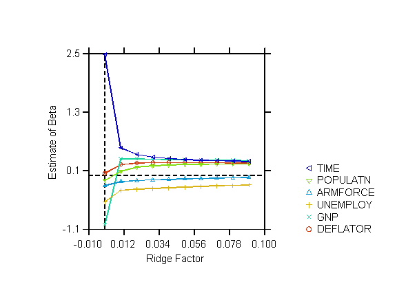
Ridge regression is based on the standardized regression model with normal equations

r_XXb* = r_YX

where r_XX is the matrix of correlations of X, r_YX are the correlations of Y with the X, and b* is the vector of standardized regression coefficients.
The ridge estimators adds a "biasing constant" c >= 0 so that the normal equations become

(r_XX+ cI)b^R = r_YX

where b^R contains the ridge coefficient estimates, so that

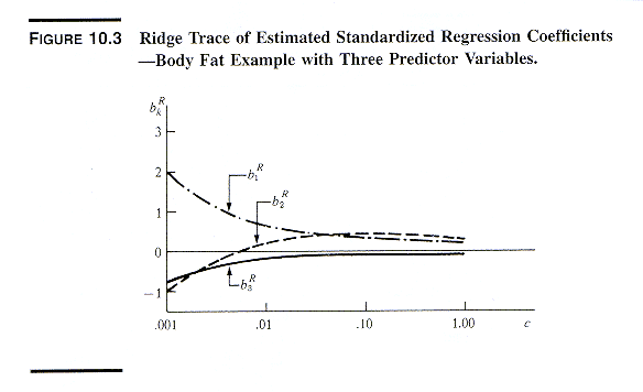
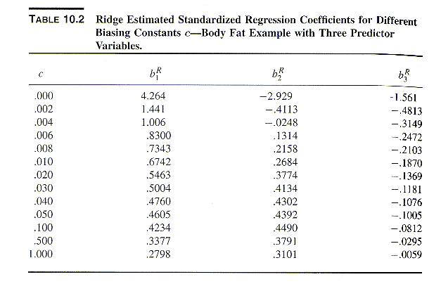
b^R = (r_XX+ cI)^-1r_YX

The strategy is to try several successive values of c starting from zero and choose the value for which

the coefficients become "stable"
the (VIF)_k become sufficiently small

This is an informal judgement based on the graph of the b^R against c called the ridge trace.
The following exhibits show an example of ridge estimation for the body fat data.

The following exhibits show a matrix procedure for ridge regression using SYSTAT's matrix module.

Once the value of c is chosen and the standardized coefficients b^R obtained, one can recover the unstandardized coefficient estimates using the formulas (NKNW 7.53a and 7.53b p. 282)

b_k = (s_Y/s_k)b_k^R (k = 1, ..., p-1)
b₀ = Y_. - b₁X_.1 - ... - b_p-1X_.,p-1

where s_Y and s_k are the sample standard deviations of Y and X_k, respectively.

Last modified 6 Apr 2006