![Exhibit: Linear functional relation - Celsius to Fahrenheit temperature conversion [m1001.gif]](m1001.gif)
![Exhibit: Curvilinear functional relation - BMI by height for constant weight (70 kg) [m15004.jpg]](m15004.jpg)
![Exhibit: A linear statistical relation - female by male life expectancy [m15002.jpg]](m15002.jpg)
![Exhibit: A curvilinear statistical relation - female life expectancy by doctors per million [m15003.jpg]](m15003.jpg)
![Exhibit: Pictorial representation of general regression model (ALSM5e F1.4 p. 7) [m1004.gif]](m1004.gif)
![Exhibit: Pictorial representation of simple linear regression model (ALSM5e F1.6 p. 12) [m1005.gif]](m1005.gif)
![Exhibit: Graph of simple linear regression of % clerks (Y) on seasonality (X) [m15001.jpg]](m15001.jpg)
![Exhibit: Vertical deviations ei of Yi from regression line involved in estimating b0 and b1 by OLS [m15010.gif]](m15010.gif)
![Exhibit: Partitioning of total deviation of Y from the mean (NWW F18.10 p. 549) [m1012.gif]](m1012.gif)
![Exhibit: Degree of statistical relationship corresponding to several values of r (NWW F18.11 p. 556) [m1016.gif]](m1016.gif)
![Exhibit: Two misunderstandings concerning correlation coefficients (ALSM5e F2.9 p. 83) [m1017.gif]](m1017.gif)
The line or curve of statistical relationship refers to the tendency of y to vary systematically as a function of x.
The second exhibit shows a situation where the regression function is linear.Exhibit: Pictorial representation of general regression model (ALSM5e F1.4 p. 7) [m1004.gif]
The regression model is the formalization of the idea of a statistical relation; it translates the idea into two components:Exhibit: Pictorial representation of simple linear regression model (ALSM5e F1.6 p. 12) [m1005.gif]
Yi = b0 + b1Xi + ei i = 1, 2, ..., n (1)where
Assumption of normality of the errors is necessary to theoretically justify statistical inference (see Module 2), especially in small samples. But most properties of least squares estimators of model parameters do not depend on the normality assumption.
E{Y} = E{b0 + b1Xi + ei} = b0 + b1Xi + E{ei} = b0 + b1Xsince by assumption E{ei} = 0.
The parameters b0
and b1
are called regression coefficients or regression parameters.
The meaning of each coefficient is as follows
s2{Yi} = s2{b0 + b1Xi + ei} = s2{ei} = s2where s2 is the variance of ei. This is because ei is the only random variable in the expression, and the variance of the error ei is assumed to be the same and equal to s2 regardless of the value of X. (This definition of the population variance of Y as s2 , i.e., the variance of ei, may be confusing as it does not corresponds directly to the sample variance of Y, Sy2 . It is helpful to consider that s2{Yi} actually means "variance of y around the regression line", so an equivalent expression for s2{Yi} is s2{Y|X}, or "variance of Y (around the regression line) given a certain value of X".)
The quantities b0 and b1 and s2 are the parameters of the regression model; they have to be estimated from the data. (In reality one estimates b0 and b1 and then the estimate of s2 is obtained as a by-product.)
|
|
Sector | Xi | Yi | (Xi - X.) | (Yi - Y.) | (Xi - X.)2 | (Yi - Y.)2 | (Xi - X.)
x (Yi - Y.) |
| 1 | STRSEW | 73 | 4.8 | 33.444 | -3.156 | 1118.531 | 9.958 | -105.536 |
| 2 | SAND | 43 | 7.6 | 3.444 | -0.356 | 11.864 | 0.126 | -1.225 |
| 3 | VENT | 29 | 11.7 | -10.556 | 3.744 | 111.420 | 14.021 | -39.525 |
| 4 | BRICK | 47 | 3.3 | 7.444 | -4.656 | 55.420 | 21.674 | -34.658 |
| 5 | GENCON | 43 | 5.2 | 3.444 | -2.756 | 11.864 | 7.593 | -9.491 |
| 6 | SHEET | 29 | 11.7 | -10.556 | 3.744 | 111.420 | 14.021 | -39.525 |
| 7 | PLUMB | 20 | 10.9 | -19.556 | 2.944 | 382.420 | 8.670 | -57.580 |
| 8 | ELEC | 13 | 12.5 | -26.556 | 4.544 | 705.198 | 20.652 | -120.680 |
| 9 | PAINT | 59 | 3.9 | 19.444 | -4.056 | 378.086 | 16.448 | -78.858 |
| Total | 356 | 71.6 | -0.000 | 0.000 | 2886.222 | 113.162 | -487.078 | |
| Mean | 39.556 | 7.956 |
The next exhibit shows a scatterplot in which each point corresponds to the pair of values (yi, xi), with y measured on the vertical axis and x measured on the horizontal axis.
The solid line is the estimated regression line. It is represented by the equationExhibit: Graph of simple linear regression of % clerks (Y) on seasonality (X) [m15001.jpg]
^y = b0 + b1xwhere ^y (called "y hat") represents the vertical coordinate of a point on the regression line corresponding to horizontal coordinate x. The coefficient b0 and b1 are calculated by the method of least squares (explained below). The model implies that for each observation in the sample the vertical coordinate yi of a point is given by the formula
yi = ^yi + ei or
yi = b0 + b1xi + ei (i = 1, ..., 9)where ei corresponds to the vertical deviation between the observed value yi and ^yi (called the fitted value or predictor of y) implied by the regression line. ei is called the residual for observation i.
Note that the simple regression model establishes an asymmetry between the dependent variable y and independent variable x, because deviations are measured along the dependent variable dimension (usually the vertical axis). In general a different regression line is obtained if one exchange y and x in their roles. The choice of one variable as dependent and the other as independent is a substantive choice. (Correlational models do not assume this asymmetry.)
Q = Si=1 to n (yi - b0 - b1xi)2The following exhibit shows the vertical deviations ei that are squared and summed up to evaluate Q. To minimize Q one could: (1) use a "brute force" numerical search using a grid of values for b0 and b1 (this is actually what computers can do in situations), or (2) take advantage of the analytical solution originally discovered by French mathematician Legendre. Legendre discovered that the values b0 and b1 that minimize Q are given by the formulas
b1 = (S(Xi - X.)(Yi - Y.))/S(Xi - X.)2
b0 = Y. - b1X.called the normal equations. All the sums are over all observations (from i=1 to n). Table 1 shows how one can organize the calculations for the construction industry data. In the table units are sectors of the construction industry, yi stands for % clerks, and xi for the index of employment seasonality. One calculates b1first, then b0. Thus having calculated the sums of squares and cross-products one calculates b0 and b1 using the formulas above as
b1 = (-487.078)/(2886.222) = -0.169Note that the slope b1 could also be calculated as the ratio of the same two numbers, each divided by n-1, i.e. as the sample covariance of x and y, denoted sxy, divided by the variance of x, denoted sx2, as
b0 = (7.956) - (-0.169)(39.556) = 14.631
b1 = sXY/sX2In practice one uses a computer program to carry out the calculations. The next exhibit shows a typical simple regression output.
b0 = Y. - b1X.
| Aspect of the Population Model | Symbolic Form | Estimate |
| Regression coefficients | b0 , b1 | b0, b1 |
| Mean response (regression function for given value Xh of X, whether or not Xh is represented in the sample) | E{Yh} = b0+ b1Xh | ^Yh = b0 + b1Xh |
| Estimate, predictor or fitted value of Y (for Xi in the sample) | E{Yi} = b0+ b1Xi | ^Yi = b0 + b1Xi |
| Predicted value of Y for known value Xh of X (Xh not necessarily in the sample) | Yh = b0+ b1Xh + e | ^Yh = b0 + b1Xh |
| Residual (Xi in the sample) | ei | ei = Yi - ^Yi |
| Residual variance (variance of ei) | s2 | MSE = SSE/(n-2) |
| Standard error of estimate (standard deviation of ei) | s | MSE1/2 |
Q = Si=1 to n (Yi - b0 - b1Xi)2can be viewed as a function of two variables, b0 and b1. To find the values of b0 and b1 that minimize Q one differentiates the function in turn with respect to b0 and with respect to b1, obtaining
dQ/db0 = -2Si=1 to n (Yi - b0 - b1Xi)The values b0 and b1 that minimize Q are found by setting the derivatives to zero, as
dQ/db1 = -2Si=1 to n Xi(Yi - b0 - b1Xi)
-2Si=1 to n (Yi - b0 - b1Xi) = 0and solving for b0 and b1. Solving is done by simplifying and expanding these equations and rearranging the terms to produce the normal equations
-2Si=1 to n Xi(Yi - b0 - b1Xi) = 0
SYi = nb0 + b1SXiOne can also derive the normal equations (although not demonstrate that their solution provides the values of b0 and b1 that minimize the sum of squared residuals) by multiplying through the equation Y=b0+b1X in turn by 1 and by X, and summing the products over all observations. This observation presages the multiple regression model seen later.
SXiYi = b0SXi + b1SXi2
Yi = ^Yi + ei i=1,...,nwhere
^Yi = b0 + b1Xiis the predictor (or fitted value, or estimate) of Yi given Yi, and
ei = Yi - ^Yiis called the residual.
|
|
|
|
|
|
|
|
|
|
Next take the sum of the squares of each deviation
over all observations in the sample.
| Sum of squares: |
|
|
|
| Name: |
|
|
|
| Meaning: |
|
|
|
SSE is also called residual sum of squares. The
basic ANOVA result (or theorem) is that the sums of squared deviations
stand in the same relation as the (unsquared) deviations, so that:
|
|
|
|
|
|
|
|
|
|
|
|
|
|
This is actually a remarkable and non-obvious property
that must be proven! (See optional proof in ALSM5e p. <>.)
Table 3 shows the calculations of ANOVA sums of squares for the regression
of % clerks (Y) on employment seasonality (X).
|
|
|
|
|
|
|
(Yi - Y.)2 | (^Yi - Y.)2 | (Yi - ^Yi)2 |
| 1 | STRSEW | 73 | 4.8 | 2.311 | 2.489 | 9.958 | 31.856 | 6.193 |
| 2 | SAND | 43 | 7.6 | 7.374 | 0.226 | 0.126 | 0.338 | 0.051 |
| 3 | VENT | 29 | 11.7 | 9.737 | 1.963 | 14.021 | 3.173 | 3.854 |
| 4 | BRICK | 47 | 3.3 | 6.699 | -3.399 | 21.674 | 1.578 | 11.555 |
| 5 | GENCON | 43 | 5.2 | 7.374 | -2.174 | 7.593 | 0.338 | 4.727 |
| 6 | SHEET | 29 | 11.7 | 9.737 | 1.963 | 14.021 | 3.173 | 3.854 |
| 7 | PLUMB | 20 | 10.9 | 11.256 | -0.356 | 8.670 | 10.891 | 0.127 |
| 8 | ELEC | 13 | 12.5 | 12.437 | 0.063 | 20.652 | 20.084 | 0.004 |
| 9 | PAINT | 59 | 3.9 | 4.674 | -0.774 | 16.448 | 10.768 | 0.599 |
| Total | 356 | 71.6 | 113.162 | 82.199 | 30.963 | |||
| Mean | 39.556 | 7.956 |
|
|
|
|||
| b1 = | -0.169 | |||||||
| b0 = | 14.631 |
Alternative computational formulas are:
|
|
|
|
|
|
|
|
|
|
||
|
|
|
b0 and b1) |
|
|
|
|
|
sample variance of y |
|
|
Mean squares total is simply the sample variance
of Y.
MSE is an estimate of the variance of the residuals
s2.
| Source | Sum of Squares | df | Mean Squares | F-ratio |
| Regression | SSR | 1 | MSR=SSR/1 | F*=MSR/MSE |
| Error | SSE | n-2 | MSE=SSE/(n-2) | |
| Total | SSTO | n-1 | s2{Y}=SSTO/(n-1) |
Table 3b shows the ANOVA table for the regression
of % clerks on employment seasonality.
| Source | Sum of Squares | df | Mean Squares | F-ratio |
| Regression | 82.199 | 1 | 82.199 | 18.583 |
| Error | 30.963 | 7 | 4.423 | |
| Total | 113.162 | 8 | 14.145 |
The F-ratio is calculated as the ratio F* = MSR/MSE (here 82.199/4.423 = 18.583); the meaning of F* is discussed in Module 2.
Q - What are the meanings of the quantities 4.423 and 14.145 in Table 3?
The ANOVA table is part of the usual regression output.
r2 = (SSTO - SSE)/SSTO = SSR/SSTO = 1 - SSE/SSTOwhere 0 <= r2 <= 1
Example: In the regression of % clerks on seasonality the r2 can be calculated equivalently as
(113.162 - 30.963)/113.162 = 82.199/113.162 = 1 - (30.963/113.162) = 0.726Limiting cases:
|r| > r2so that the absolute value of r is always larger than r2. Thus r suggests a stronger relationship and thus has a greater psychological impact than that of r2. An example is the regression of % clerks on seasonality where the r2 is 0.726 and the correlation coefficient r is a more impressive -.852.
Examples of the degree of association corresponding to various values of r are shown in the next exhibit.
The correlation coefficient r alone can give a misleading idea of the nature of a statistical relationship, so it is important to always look at the scatterplot of the relationship.b1* = b1(sX/sY)i.e., b1* is equal to b1 multiplied by the standard deviation of X and divided by the standard deviation of Y. Thus in the simple linear regression model the standardized regression coefficient is the same as the correlation coefficient:
b1* = (sXY/sX2)(sX/sY) = sXY/(sXsY) = rbut this is no longer true in the multiple regression model.
b1 = b1*(sY/sX) ( = r(sY/sX), in simple linear regression only)where sX and sY are the sample standard deviations of X and Y, respectively.
In the construction industry study the regression coefficient b1 is -.169; the standard deviations of X and Y are 18.994 and 3.761, respectively. Thus the standardized coefficient of seasonality is -.169(18.944/3.761) = -.852. Thus an increase of in SD in X is associated with a decrease of .852 SD deviation of Y. (The standardized coefficient can also be automatically computed by the statistical program.)
Standardized coefficients are found in many statistical contexts, including multiple regression models and structural equations models. Calculating the standardized coefficient from the unstandardized coefficient, and vice-versa, is always done the same way. Suppose the unstandardized coefficient b of the regression of a variable Y on a variable X is represented as
X -- b --> YThen
Example: Brody (1992: 253) reports a correlation of .57 between 6th grade IQ test score and the number of years of education that a person obtained. One can interpret this correlation as a standardized regression coefficient: b* = .57 means that an individual with a 6th grade IQ score 1 SD above the mean would be expected to obtain .57 SD years of education above the mean.The following picture shows an interpretation of b1* as a shift along distribution of years of education caused by a positive shift of 1 SD of IQ from the mean. Standardized coefficients are especially useful in the multiple regression model, where they permit comparing the relative magnitudes of the coefficients of independent variables measured in different units (such as a variable measured in years, and another measured in thousands of dollars).
Data for regression analysis comes from two kinds of sources.
Compare the following two studies with respect to the strength of causal inference.
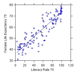
Example of observational data: Regression of female life expectancy on literacy rate for countries
Estimated regression: Y = 36.212 + .377X R2=.844 N=131
Example of experimental data: Shepard's experiment
"The data are from a perceptual experiment in which subjects viewed pairs of objects differing only by rotational angle. [...] The rt variable is reaction time (delay in saying "same" for a pair). [...] Shepard's remarkable discovery in this and other experiments was that the rotational angle is linearly related to reaction time. The February 19, 1971 cover of Science magazine displayed five of Shepard's computer-generated images under various rotations. This research has been replicated by psychologists and neuroscientists studying spatial processing in humans and other primates. Shepard received the National Medal of Science for this and other work in cognitive psychology." (Wilkinson 1999, p. 337.)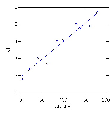
Estimated regression: RT = 1.916 + (.021)ANGLE
R2 = .949 N=10
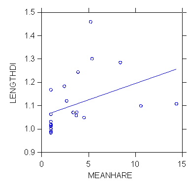
>rem relationship
berween sex dimorphism (length ratio male to female) and
>rem mean harem size
in primates, a measure of sexual competition among males
>rem ask me for the whole
bizarre story
>regress
>model lengthdi=constant+meanhare
>estimate
Dep Var: LENGTHDI N: 22 Multiple R: 0.403 Squared multiple R: 0.162
Adjusted squared multiple R: 0.120 Standard error of estimate: 0.115
Effect
Coefficient Std Error Std Coef
Tolerance t P(2 Tail)
CONSTANT
1.055 0.035
0.000 . 29.949
0.000
MEANHARE
0.014 0.007
0.403 1.000 1.967
0.063
Analysis of Variance
Source
Sum-of-Squares df Mean-Square
F-ratio P
Regression
0.051 1
0.051 3.870
0.063
Residual
0.266 20 0.013
-------------------------------------------------------------------------------
*** WARNING ***
Case
17 has large leverage (Leverage =
0.487)
Case
19 is an outlier (Studentized
Residual = 3.821)
Durbin-Watson D Statistic
1.949
First Order Autocorrelation
-0.026
>plot lengthdi*meanhare/stick=out smooth=linear short
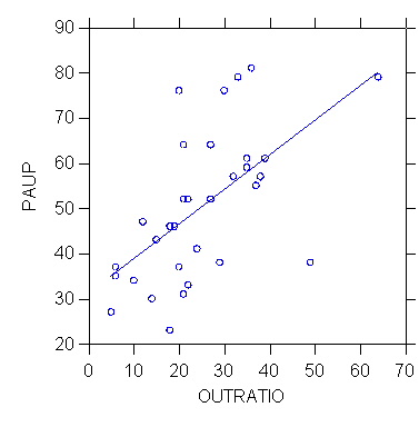
>USE "Z:\mydocs\ys209\yule.syd"
SYSTAT Rectangular file
Z:\mydocs\ys209\yule.syd,
created Wed Feb 17,
1999 at 09:34:32, contains variables:
UNION$
PAUP OUTRATIO
PROPOLD POP
>model paup=constant+outratio
>estimate
Dep Var: PAUP
N: 32 Multiple R: 0.594 Squared multiple R: 0.353
Adjusted squared multiple
R: 0.331 Standard error of estimate: 13.483
Effect
Coefficient Std Error Std Coef
Tolerance t P(2 Tail)
CONSTANT
31.089 5.324
0.000 .
5.840 0.000
OUTRATIO
0.765 0.189
0.594 1.000 4.045
0.000
Analysis of Variance
Source
Sum-of-Squares df Mean-Square
F-ratio P
Regression
2973.751 1 2973.751
16.359 0.000
Residual
5453.468 30 181.782
-------------------------------------------------------------------------------
*** WARNING ***
Case
15 has large leverage (Leverage =
0.328)
Durbin-Watson D Statistic
1.853
First Order Autocorrelation
-0.018
>plot paup*outratio/stick=out smooth=linear short
. use "Z:\mydocs\S208\gss98.dta", clear
. su income
Variable
| Obs
Mean Std. Dev. Min
Max
-------------+-----------------------------------------------------
income | 2699 10.85624
2.429604 1
13
. su educ
Variable
| Obs
Mean Std. Dev. Min
Max
-------------+-----------------------------------------------------
educ | 2820 13.25071 2.927512
0 20
. regress income educ
Source | SS
df MS
Number of obs = 2688
-------------+------------------------------
F( 1, 2686) = 235.66
Model | 1269.91329 1 1269.91329
Prob > F = 0.0000
Residual
| 14474.0495 2686 5.38870049
R-squared = 0.0807
-------------+------------------------------
Adj R-squared = 0.0803
Total | 15743.9628 2687 5.85930882
Root MSE = 2.3214
------------------------------------------------------------------------------
income | Coef. Std. Err.
t P>|t| [95% Conf. Interval]
-------------+----------------------------------------------------------------
educ | .2359977 .0153731 15.35
0.000 .2058533 .2661421
_cons | 7.71967 .2094621
36.85 0.000 7.308947
8.130393
------------------------------------------------------------------------------
![Exhibit: Picture of Adrien Legendre (1752-1833) (Stigler 1986 p. 11) [m1010.gif]](m1010.gif)
![Exhibit: Legendre's appendix (1805) on the method of least squares (Stigler 1986, Figure 1.5 p. 58) [m1011.gif]](m1011.gif)
![Exhibit: Picture of Francis Galton (1822-1911) (Stigler 1986 p. 265) [m1023.jpg]](m1023.jpg)
![Exhibit: Galton's cross-tabulation of child's height by midparent's height (Stigler 1986, Table 8.1 p. 286) [m1021.jpg]](m1021.jpg)
![Exhibit: Origin of the term regression: "regression to mediocrity" of child's height relative to midparent's height (Stigler 1986, Figure 8.8 p. 295) [m1022.jpg]](m1022.jpg)
![Exhibit: Data on stature by left cubit length used by Galton to calculate the first published correlation coefficient in 1888 (Stigler 1986, Table 9.1 p. 319 [m1024.jpg]](m1024.jpg)
![Exhibit: The first published correlation (Stigler 1986, Figure 9.2 p. 320) [m1025.jpg]](m1025.jpg)