File D:\MYDOCS\YS209\DEPRES1.SYD
>USE "D:\mydocs\ys209\survey2a.syd"
SYSTAT
Rectangular file D:\mydocs\ys209\survey2a.syd,
created
Tue Apr 18, 2000 at 09:50:17, contains variables:
ID
SEX AGE
MARITAL EDUCATN
EMPLOY
INCOME
RELIGION BLUE
DEPRESS LONELY
CRY
SAD
FEARFUL FAILURE
AS_GOOD HOPEFUL
HAPPY
ENJOY
BOTHERED NO_EAT
EFFORT BADSLEEP
GETGOING
MIND
TALKLESS UNFRNDLY DISLIKE
TOTAL CASECONT
DRINK
HEALTHY DOCTOR
MEDS BED_DAYS
ILLNESS
CHRONIC
MARITAL$ SEX$
AGE$ EDUC$
FEMALE
CATH
JEWI NONE
L10INC
>mglh
>model
total=constant+age+female+l10inc+educatn+cath+jewi+none
>save
depres1/model
>estimate
Dep
Var: TOTAL N: 256 Multiple R: 0.378694
Squared multiple R: 0.143409
Adjusted
squared multiple R: 0.119231 Standard error of estimate: 8.361515
Effect Coefficient Std Error Std Coef Tolerance t P(2 Tail)
CONSTANT
19.776246 3.083963 0.000000
. 6.41261 0.00000
AGE
-0.080870 0.033446 -0.145591
0.952675 -2.41794 0.01633
FEMALE
2.475360 1.091627 0.136720
0.950133 2.26759 0.02422
L10INC
-5.842862 1.826501 -0.204619
0.844191 -3.19894 0.00156
EDUCATN
-0.766779 0.436350 -0.112592
0.841352 -1.75726 0.08011
CATH
0.940902 1.438833 0.040625
0.894977 0.65393 0.51376
JEWI
4.955468 1.915932 0.159361
0.909842 2.58645 0.01027
NONE
3.544925 1.403983 0.160391
0.855958 2.52491 0.01220
Analysis of Variance
Source
Sum-of-Squares df Mean-Square
F-ratio P
Regression
2902.844806 7 414.692115
5.931381 0.000002
Residual
1.73389E+04 248 69.914940
***
WARNING ***
Case
216 is an outlier (Studentized
Residual = 3.751558)
Case
220 is an outlier (Studentized
Residual = 4.040754)
Case
256 is an outlier (Studentized
Residual = 4.586381)
Durbin-Watson
D Statistic 0.725
First
Order Autocorrelation 0.599
Residuals
have been saved.
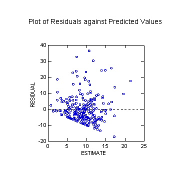
Plot
of Residuals against Predicted Values
File
D:\MYDOCS\YS209\DEPRES1.SYD
>USE "D:\mydocs\ys209\depres1.SYD"
SYSTAT
Rectangular file D:\mydocs\ys209\depres1.SYD,
created
Tue Apr 18, 2000 at 09:53:38, contains variables:
ESTIMATE
RESIDUAL LEVERAGE COOK
STUDENT SEPRED
TOTAL
X(1..7)
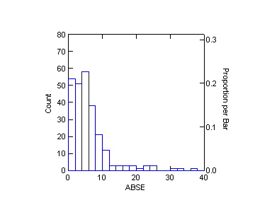
>let
abse=abs(residual)
>let
sqe=residual^2
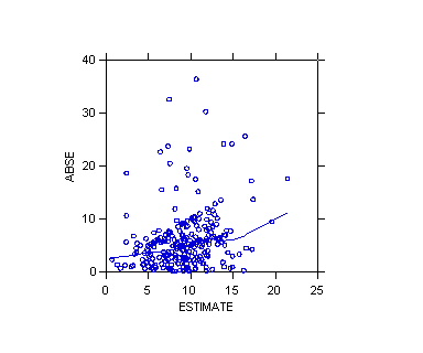
>plot
abse*estimate/stick smooth=lowess
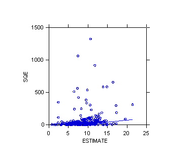
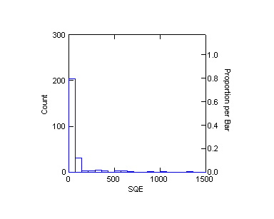
>plot
sqe*estimate/stick smooth=lowess
>corr
>pearson estimate abse sqe
Pearson correlation matrix
ESTIMATE ABSE
SQE
ESTIMATE
1.000000
ABSE
0.244210 1.000000
SQE
0.169025 0.919364 1.000000
Number of observations: 256
>mglh
>model
abse=constant+estimate
>estimate
Dep
Var: ABSE N: 256 Multiple R: 0.244210
Squared multiple R: 0.059639
Adjusted
squared multiple R: 0.055936 Standard error of estimate: 5.492641
Effect
Coefficient Std Error Std Coef
Tolerance t P(2 Tail)
CONSTANT
2.245065 0.994566 0.000000
. 2.25733 0.02484
ESTIMATE
0.409169 0.101946 0.244210
1.000000 4.01359 0.00008
Analysis of Variance
Source
Sum-of-Squares df Mean-Square
F-ratio P
regression
485.991719 1 485.991719
16.108918 0.000079
Residual
7662.953848 254 30.169110
***
WARNING ***
Case
216 is an outlier (Studentized
Residual = 4.386271)
Case
220 is an outlier (Studentized
Residual = 5.229236)
Case
256 is an outlier (Studentized
Residual = 5.766427)
Durbin-Watson
D Statistic 1.066
First
Order Autocorrelation 0.409
Plot of Residuals against Predicted Values
>let
shat=2.245065+0.409169*estimate
>let
w=1/shat^2
>weight=w
>model
total=constant+x(1)+x(2)+x(3)+x(4)+x(5)+x(6)+x(7)
>estimate
Dep
Var: TOTAL N: 256 Multiple R: 0.339960
Squared multiple R: 0.115573
Adjusted
squared multiple R: 0.090609 Standard error of estimate: 1.383587
Effect
Coefficient Std Error Std Coef
Tolerance t P(2 Tail)
CONSTANT
16.180076 2.990710 0.000000
. 5.41011 0.00000
X(1)
-0.061528 0.031496 -0.119452
0.953800 -1.95351 0.05188
X(2)
2.395679 0.981830 0.151064
0.930405 2.44001 0.01539
X(3)
-4.495666 1.795997 -0.168512
0.786909 -2.50316 0.01295
X(4)
-0.449962 0.377421 -0.080274
0.786607 -1.19220 0.23432
X(5)
2.041598 1.283965 0.099145
0.917283 1.59007 0.11309
X(6)
3.335261 2.006405 0.102181
0.943827 1.66231 0.09771
X(7)
2.966680 1.407609 0.132249
0.905739 2.10760 0.03607
Analysis of Variance
Source
Sum-of-Squares df Mean-Square
F-ratio P
Regression
62.038105 7 8.862586
4.629645 0.000069
Residual
474.749500 248 1.914313
-------------------------------------------------------------------------------
***
WARNING ***
Case
1 has large leverage (Leverage = 0.340706)
Case
2 has large leverage (Leverage = 0.268667)
Case
3 has large leverage (Leverage = 0.334971)
Case
3 is an outlier (Studentized
Residual = -4.265162)
... Many, many lines deleted for the sake of space; SYSTAT seems to have a quirk that produces zillions of warnings in weighted regressions.
Case
254 is an outlier (Studentized
Residual = 9.719915)
Case
255 has large leverage (Leverage =
1.140177)
Case
256 has large leverage (Leverage =
0.805603)
Case
256 has large influence (Cook distance = 1912.626896)
Durbin-Watson
D Statistic 0.680
First
Order Autocorrelation 0.621
Plot of Residuals against Predicted Values
>list total estimate residual shat w/n=10
Case number TOTAL
ESTIMATE RESIDUAL
SHAT
W
1 4.000000
4.983149 -0.983149 4.284015
0.054488
2 4.000000
7.767519 -3.767519 5.423293
0.034000
3 5.000000
10.064895 -5.064895 6.363308
0.024696
4 6.000000
8.189291 -2.189291 5.595869
0.031935
5 7.000000
9.229516 -2.229516 6.021497
0.027580
6 15.000000
9.722067 5.277933 6.223033
0.025822
7 10.000000
9.853902 0.146098 6.276976
0.025380
8 0.000000
10.268245 -10.268245 6.446513
0.024063
9 4.000000
7.173695 -3.173695 5.180319
0.037264
10 8.000000
6.544159 1.455841 4.922732
0.041266
Weighting does not do much good in this case, probably because the standard error function has such low fit.