SYSTAT
Rectangular file D:\mydocs\ys209\yule.syd,
created
Wed Feb 17, 1999 at 09:34:32, contains variables:
UNION$ PAUP OUTRATIO PROPOLD POP
>rem
first use mglh to do a regular regression and save residuals to
>rem
identify any influential case
>mglh
>model
paup=constant+outratio+propold+pop
>save
yuleres1/data
>estimate
Dep
Var: PAUP N: 32 Multiple R: 0.835 Squared
multiple R: 0.697
Adjusted
squared multiple R: 0.665 Standard error of estimate: 9.547
Effect
Coefficient Std Error Std Coef
Tolerance t P(2 Tail)
CONSTANT
63.188 27.144
0.000 .
2.328 0.027
OUTRATIO
0.752 0.135
0.584 0.985 5.572
0.000
PROPOLD
0.056 0.223
0.031 0.711 0.249
0.805
POP
-0.311 0.067
-0.570 0.719 -4.648
0.000
Analysis of Variance
Source
Sum-of-Squares df Mean-Square
F-ratio P
Regression
5875.320 3 1958.440
21.488 0.000
Residual
2551.899 28 91.139
***
WARNING ***
Case
15 has large leverage (Leverage =
0.424)
Case
30 is an outlier (Studentized
Residual = 3.618)
Durbin-Watson
D Statistic 2.344
First
Order Autocorrelation -0.177
Residuals
have been saved.
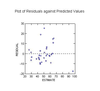
-------------------------------------------------------------------------------
Plot of Residuals against Predicted Values
>use yuleres1
SYSTAT
Rectangular file d:\MYDOCS\YS209\yuleres1.SYD,
created
Wed Apr 26, 2000 at 20:39:58, contains variables:
ESTIMATE
RESIDUAL LEVERAGE COOK
STUDENT SEPRED
UNION$
PAUP OUTRATIO
PROPOLD POP
>plot cook/stick line dash=11
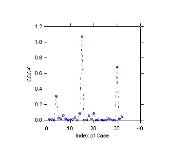
>rem
calculate percentiles of the f(p, n-p) distribution
>let
fperc=100*fcf(cook,4,28)
>rem
#4 is 12.9%, #15 61.0%, #30 38.9%; 15 and 30 are influential
>use
yule
SYSTAT
Rectangular file d:\MYDOCS\YS209\yule.SYD,
created
Wed Feb 17, 1999 at 09:34:32, contains variables:
UNION$ PAUP OUTRATIO PROPOLD POP
>model
paup=constant+outratio+propold+pop
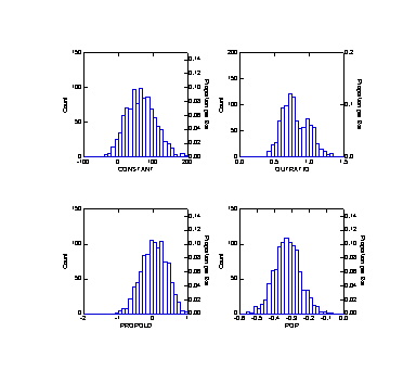
>rem
now do a bootstrap of the ordinary regression
>output/noscreen
** following three lines are not echoed because of the "noscreen"
>save yulebot1/coef
>estimate/sample=boot(1000,32)
>output
** bootstrap took 14s on my 266MHz machine at home
>use
yulebot1
SYSTAT
Rectangular file d:\MYDOCS\YS209\yulebot1.SYD,
created
Wed Apr 26, 2000 at 20:50:58, contains variables:
CONSTANT OUTRATIO PROPOLD POP
>den constant..pop
>stats
>stat
constant..pop
CONSTANT OUTRATIO PROPOLD POP
N of cases
1000 1000
1000 1000
Minimum
-35.597 0.286
-1.007 -0.555
Maximum
194.383 1.365
0.922 -0.076
Mean
65.935 0.802
0.033 -0.325
Standard Dev 41.621
0.188 0.357
0.074
>rem
compare "naive" bootstrap estimates of se with original ols regression
>use
yule
SYSTAT
Rectangular file d:\MYDOCS\YS209\yule.SYD,
created
Wed Feb 17, 1999 at 09:34:32, contains variables:
UNION$ PAUP OUTRATIO PROPOLD POP
>rem
now try robust estimation
>nonlin
>model
paup=b0+b1*outratio+b2*propold+b3*pop
>robust
bisquare=3.5
>estimate
Iteration
No.
Loss B0
B1 B2
B3
0 .334285D+04 .160251D+02 .942626D+00 .461206D+00-.309542D+00
1 .171546D+03 .631877D+02 .752095D+00 .556020D-01-.310738D+00
2 .438515D+03 .627919D+02 .778592D+00 .431065D-01-.311909D+00
3 .323610D+03 .489783D+02 .863971D+00 .132061D+00-.295710D+00
4 .282858D+03 .406098D+02 .874491D+00 .193804D+00-.282241D+00
5 .272693D+03 .368503D+02 .878163D+00 .224339D+00-.277979D+00
6 .290391D+03 .352696D+02 .880899D+00 .238965D+00-.277741D+00
7 .294784D+03 .354647D+02 .881415D+00 .238072D+00-.278577D+00
8 .291739D+03 .356665D+02 .881671D+00 .236611D+00-.279004D+00
9 .289610D+03 .355798D+02 .881851D+00 .237442D+00-.279020D+00
10 .289554D+03 .354608D+02 .882028D+00 .238572D+00-.279026D+00
11 .289789D+03 .354197D+02 .882160D+00 .239034D+00-.279096D+00
12 .289680D+03 .354128D+02 .882244D+00 .239166D+00-.279161D+00
13 .289484D+03 .354026D+02 .882301D+00 .239298D+00-.279196D+00
14 .289383D+03 .353892D+02 .882343D+00 .239445D+00-.279215D+00
15 .289345D+03 .353796D+02 .882374D+00 .239551D+00-.279230D+00
16 .289315D+03 .353741D+02 .882397D+00 .239617D+00-.279243D+00
17 .289286D+03 .353704D+02 .882412D+00 .239661D+00-.279252D+00
18 .289264D+03 .353675D+02 .882424D+00 .239694D+00-.279258D+00
19 .289250D+03 .353653D+02 .882432D+00 .239719D+00-.279263D+00
20 .289240D+03 .353637D+02 .882438D+00 .239737D+00-.279266D+00
21 .289233D+03 .353627D+02 .882442D+00 .239750D+00-.279268D+00
22 .289227D+03 .353619D+02 .882445D+00 .239759D+00-.279270D+00
23 .289224D+03 .353613D+02 .882447D+00 .239765D+00-.279271D+00
24 .289221D+03 .353609D+02 .882449D+00 .239770D+00-.279272D+00
25 .289219D+03 .353606D+02 .882450D+00 .239773D+00-.279272D+00
BISQUARE
robust regression: 27 cases have positive psi-weights
The average psi-weight is 0.83243
Dependent variable is PAUP
Zero weights, missing data or estimates reduced degrees of freedom
Source Sum-of-Squares df Mean-Square
Regression
86611.288 4 21652.822
Residual 2919.712
23 126.944
Total 89531.000 27
Mean
corrected 8427.219 26
Raw R-square (1-Residual/Total)
= 0.967
Mean
corrected R-square (1-Residual/Corrected) =
0.654
R(observed vs predicted) square =
0.686
Wald Confidence Interval
Parameter
Estimate A.S.E. Param/ASE
Lower < 95%> Upper
B0
35.361 40.768
0.867 -48.975
119.696
B1
0.882 0.207
4.264 0.454
1.311
B2
0.240 0.343
0.699 -0.470
0.950
B3
-0.279 0.096
-2.915 -0.477
-0.081
>rem
se for outratio is now 0.207, but this is based on asymptotic
>rem
theory, i.e. justified for large samples; use bootstrap as
>rem
alternative approach to inference
>model
paup=b0+b1*outratio+b2*propold+b3*pop
>robust
bisquare=3.5
>output/noscreen
**
following 3 lines not echoed because of the "noscreen"
>save yulebot2/params
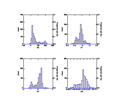
>estimate/sample=boot(1000,32)
>output
>rem
bootstrap took 1m 33s on my 266MHz machine at home (OLS was 14 s)
>use
yulebot2
SYSTAT
Rectangular file d:\MYDOCS\YS209\yulebot2.SYD,
created
Wed Apr 26, 2000 at 21:07:56, contains variables:
B0 B1 B2 B3
>den b0..b3
>stats
>stat
b0..b3
B0 B1 B2 B3
N of cases
1000 1000
1000 1000
Minimum
-83.456 0.119
-1.353 -0.723
Maximum
264.132 1.678
1.258 0.038
Mean
62.969 0.880
0.027 -0.326
Standard Dev 61.126
0.214 0.484
0.124
>rem
try still another estimate of se as 1/2 width of 68% central strip
** cf Diaconis & Efron Sci. Am. paper
>basic
File
in use is d:\MYDOCS\YS209\yulebot2.SYD.
Variables
in the SYSTAT Rectangular file are:
B0 B1 B2 B3
BASIC statements cleared.
>sort b1
1000 cases and 4 variables processed.
>if
case=160 then print "68% CI LB:",b1
>if
case=840 then print "68% CI UB:",B1
>run
68%
CI LB: 0.632
68%
CI UB: 1.041
SYSTAT file created.
1000 cases and 4 variables processed.
BASIC statements cleared.
>calc
(1.041-0.632)/2
0.204
>rem
this estimate of se of b1 is 0.204, close to 0.214 (naive) and 0.207 (A.S.E)
>corr
>pearson
b0..b3
Pearson correlation matrix
B0 B1 B2 B3
B0
1.000
B1
-0.181 1.000
B2
-0.985 0.178
1.000
B3
-0.806 -0.138
0.707 1.000
Number of observations: 1000