Module 6 - POLYNOMIAL REGRESSION & INTERACTIONS

1.  POLYNOMIAL REGRESSION WITH ONE PREDICTOR VARIABLE

1.  Formulation of the Model

A nonlinear relationship between y and x can often be approximately represented within the general linear model as a polynomial function of x.
Example:

y_i  = b₀ + b₁x_i + b₂x_i² + e_i

y_i  = b₀ + b₁x_i1 + b₂x_i2 + e_i

The order of the polynomial function is the highest exponent of x; the model above is a second-order model.

To estimate a polynomial function x is often first deviated from its mean (or median) to reduce collinearity between x and higher powers of x.   A variable deviated from its mean is called centered.  The transformation is x = X - X_. where x (lower case) represents the centered variable and X (uppercase) the original (uncentered) variable.
A polynomial function can be used when

• the true response function is polynomial
• the true response function is unknown but a polynomial is a good approximation of its shape

2.  Graphic Representation of the Model

The response function E{y} for any polynomial model with one predictor variable can be represented on a 2-dimensional plot of y against x.

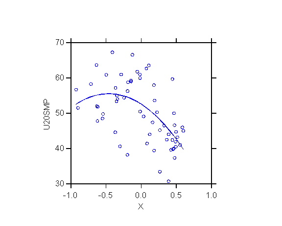
A second degree polynomial implies a parabolic relationship.  The signs of the coefficients determine the shape of the response function:

• when b₂ is positive, y increases as the value of x increases
• when b₂ is negative, y eventually decreases as the value of x increases

as shown in these graphs:

• Exhibit:  Examples of second-order polynomial response functions  (NKNW Figure 7.4 p. 297)

Example:  The Kuznets curve postulates an inverted U-shaped relationship between income inequality and economic development (measured as log GDP per capita in this example).  This curvilinear relationship is often approximated with a second degree polynomial (aka quadratic function).

• Exhibit:  Regression commands and output for polynomial model of income inequality
• Exhibit:  Plot of income inequality by GDP per capita with fitted quadratic curve

Higher degree polynomials produce curves with more inflection points:

• Exhibit:  Examples of third-order polynomial response functions  (NKNW Figure 7.5 p. 298)

When estimating a polynomial function, it is often useful to test for the joint significance of the coefficients of x, x², and higher powers of x, in addition to testing for the significance of each coefficient separately.  In a joint test of significance one tests H₀: b₁ = b₂ = 0 against the alternative that at least one of the coefficient is not zero.  Joint significance tests are explained in Module 8.

NOTES

• when evaluating the shape of a polynomial response function, it is necessary to keep within the range of x in the data, as extrapolating beyond this range may lead to misleading predictions
• it is possible to convert from the coefficients of the centered model (involving x) to the non-centered model involving the original X (see ALSM5e p. 299; ALSM4e p. 301); however, the conversion is rarely needed for substantive purposes.
• with a second-order polynomial the coefficient of x² (x centered) is the same as that of X² (X uncentered)
• fitting a polynomial regression with powers higher than three is rarely done as the interpretation of the coefficients becomes difficult and interpolation tends to become erratic.  (A polynomial of order n-1 can always be fitted exactly to n points.)
• polynomial regression models are often fitted with the hierarchical approach in which higher powers are introduced one at a time and tested for significance, and if a term of a high order is included (say, x³) then all terms of lower order (x and x²) are also included.

2.  POLYNOMIAL REGRESSION WITH MORE THAN ONE PREDICTOR VARIABLE

1. Formulation of the Model

A second-order model with two predictors has the general response function

E{Y} = b₀ + b₁x₁ + b₂x₂ + b₁₁x₁² + b₂₂x₂² + b₁₂x₁x₂

x₁ = X₁ - X_.1
x₂ = X₂ - X_.2

2.  Graphic Representation of the Model

The response function E{y} of a polynomial regression model of any order with two predictor variables may be represented in 3-dimensional space with dimensions y, x₁, and x₂.  The response function defines a surface in 3-dimensional space which can alternatively be represented

• in perspective as a surface in 3-dimensional space
• by contour curves in 2-dimensional (x₁, x₂) space representing the combinations of x₁ and x₂ that yield the same value of the response y, similar to level curves in topographical maps
• by conditional effects plots in 2-dimensional (y, x₁) space representing plots of y against x₁ for (a few) different values of x₂

Example: the model with response function

E{y} = 1,740 - 4x₁² - 3x₂² - 3x₁x₂

• Exhibit:  Quadratic response surface E{y} = 1,740 - 4x₁² - 3x₂² - 3x₁x₂  (NKNW Figure 7.6 p. 299)

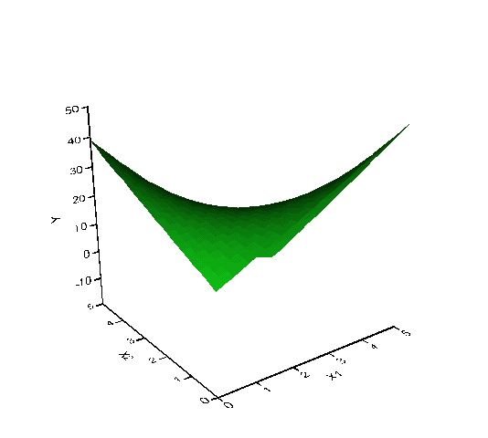
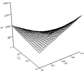
The following exhibit (figure b) is another example of a quadratic surface

• Exhibit:  Examples of response functions with 2 predictors  (NKNW Figure 6.2 p. 225)

Polynomial models involving more than 2 predictor variables are possible but the response function can no longer be represented in 3-dimensional space.

3.  INTERACTION REGRESSION MODELS

1.  Formulation of the Model

A regression model with p-1 predictors is called additive if the response function can be written in the form

E{y} = f₁(x₁) + f₂(x₂) + ... + f_p-1(x_p-1)

E{y} = b₀ + b₁x₁ + b₂x₂ + b₃x₁x₂

b₁ + b₃x₂

b₂ + b₃x₁

dE{y}/dx₁ = b₁ + b₃x₂
dE{y}/dx₂ = b₂ + b₃x₁

Example: compare the additive model

(a) E{y} = 10 + 2x₁ + 5x₂

(b) E{y} = 10 + 2x₁ + 5x₂ + 0.5x₁x₂  (reinforcement effect)
(c) E{y} = 10 + 2x₁ + 5x₂ - 0.5x₁x₂  (interference effect)

2. Graphic Representation of the Model

Interactions can be represented as plots of y against x₁ conditional on the value of x₂ called conditional effects plots:

• Exhibit:  Reinforcement & interference interaction effects  (NKNW Figure 7.10 p. 310)

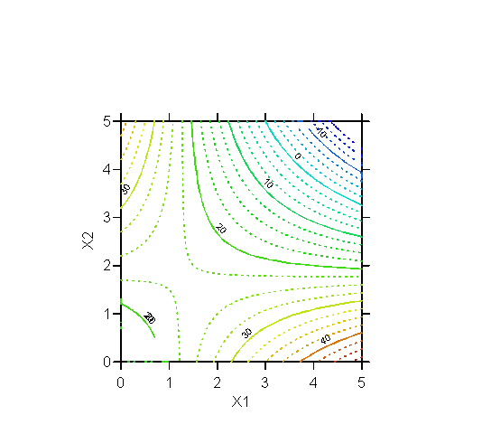
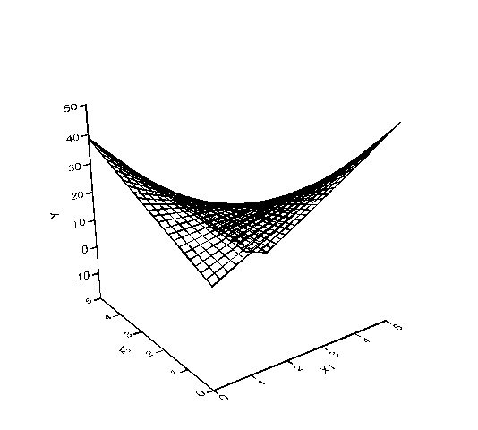
Interaction effects can also be represented by drawing the response surface (y as function of x₁ and x₂) in perspective in 3-dimensional space or using contour plots.

• Exhibit:  Response surfaces and contour plots for additive & interaction models  (NKNW Figure 7.11 p. 312)

The following exhibits show how to plot a response surface using SYSTAT and 3 representations of the interaction model of NKNW Problem 7.39 p. 323.  (As of V.9 STATA does not do 3-dimensional plots.)

• Exhibit:  SYSTAT commands for NKNW Problems 7.38 & 7.39 p. 323
• Exhibit:  Plot for NKNW 7.39 p. 323 - color
• Exhibit:  Plot for NKNW 7.39 p. 323 - contour
• Exhibit:  Plot for NKNW 7.39 p. 323 - xycut (B&W grid)

Example: (From von Eye and Schuster. 1998.  Regression Analysis for Social Science.  New York: Academic Press. Pp. 159-162.)

The authors report a regression analysis with variables

REC: Recall performance (dependent variable)
CC1: Cognitive complexity measure
EDUC: Educational background

The estimated model is (t-ratios in parentheses):