INCOME INEQUALITY & DUALISM
François Nielsen
Department of Sociology
University of North Carolina Chapel Hill
What Is Inequality?
Inequality is a property of the distribution in a population of some (presumably
valued) resource such as income or wealth but also cattle, wives (in a
polygynous society), and articles published by scholars in scientific journals.
The distribution of such quantities is typically highly skewed, with a
long tail to the right.
One can conceptualize inequality with the Lorenz curve.
Take the example of income. Imagine that all income-receiving units
(IRUs) are ranked by income from the smallest to the largest, and calculate
the cumulative share of income accruing to each category of the populations
from poorest to richest, as in the following table.
Family Income Distribution: U.S. 1983 (from Kerbo 2000, Table
2-7)
| Income Category |
Share of Total Income (%) |
p = Cumulative Share of Population (%) |
L = Cumulative Share of Income (%) |
| Top 20% |
42.7 |
100 |
100.0 |
| 4th 20% |
24.4 |
80 |
57.3 |
| 3rd 20% |
17.1 |
60 |
32.9 |
| 2nd 20% |
11.1 |
40 |
15.8 |
| Lowest 20% |
4.7 |
20 |
4.7 |
| Total |
100 |
|
|
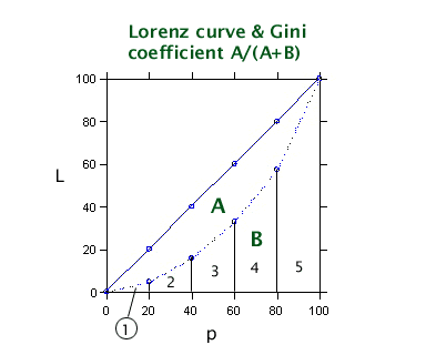
The Lorenz curve is the plot of the cumulative income share L
against the cumulative population share p.
Can One Measure Inequality?
Yes. One common measure of inequality is the Gini coefficient.
The Gini coefficient (or "Gini index" or "Gini ratio") G is calculated
from the Lorenz curve as the ratio
G = Area A/(Area A + Area B)
Note that (Area A + Area B) is the area of a triangle, given by 100*100/2=5000.
The Gini coefficient for the 1983 U.S. family income distribution is
given by the following calculations.
Calculation of Gini Coefficient
| Area A + Area B |
100*100/2 = |
5000 |
| Area 1 |
20*4.7/2 = |
47 |
| Area 2 |
20*(4.7+15.8)/2 = |
205 |
| Area 3 |
20*(15.8+32.9)/2 = |
487 |
| Area 4 |
20*(32.9+57.3)/2 = |
902 |
| Area 5 |
20*(57.3+100)/2 = |
1573 |
| Total Area B |
|
3214 |
| Area A |
5000 - 3214 = |
1786 |
| Gini Coefficient |
1786/5000 = |
0.36 or 36% |
Thus the Gini coefficient in this example is 1786/5000 = 0.36 or 36%.
In the Lorenz curve the 45 degrees line represents a situation of perfect
equality. (Why?).
In general, the closer the Lorenz curve is to the line of perfect equality,
the less the inequality and the smaller the Gini coefficient.
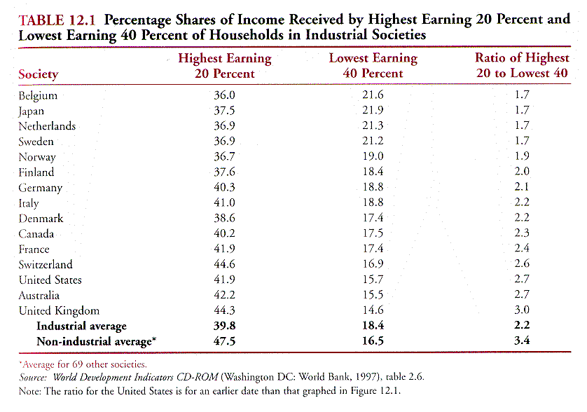
Countries differ in the inequality of their income distribution.
Note how the Lorenz curves of different countries can intersect; this means
that 2 societies with the same Gini ratio can have different Lorenz curves
(i.e., more inequality "at the bottom" versus more inequality "at the top").
Thus the Gini coefficient is not a complete description of the income distribution.
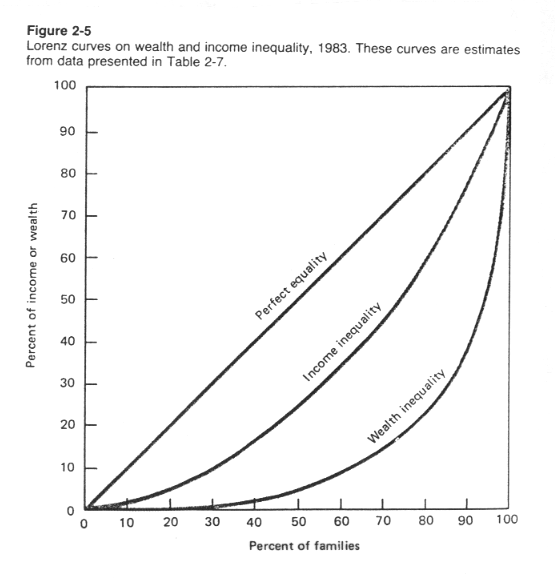
The following table shows the distribution of family wealth in the
U.S. in 1983. You may want to calculate the Gini coefficient as an
exercise.
Family Wealth Distribution: U.S. 1983 (from Kerbo 2000, Table
2-7)
| Income Category |
Share of Total Wealth (%) |
p = Cumulative Share of Population (%) |
L = Cumulative Share of Wealth (%) |
| Top 20% |
78.7 |
100 |
100.0 |
| 4th 20% |
14.5 |
80 |
21.4 |
| 3rd 20% |
6.2 |
60 |
6.9 |
| 2nd 20% |
1.1 |
40 |
0.7 |
| Lowest 20% |
-0.4 |
20 |
-0.4 |
| Total |
100 |
|
|
Inequality tends to be greater for wealth than for income. (Why?).
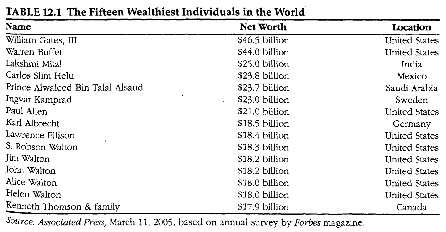
The fifteen wealthiest people in the world in 2005
Are There Other Ways to Measure Inequality?
Yes. Other more or less sophisticated measures of inequality include
the following
-
Share of total income accruing to the top 20% of IRUs; this is 42.7 for
U.S. family income distribution in 1983; share of the top 10%, or 5% are
also used; the larger, the more unequal the distribution
-
Share of total income accruing to the bottom 40% of IRUs; this is 15.8
for U.S. family income distribution in 1983; the larger, the less unequal
the distribution
-
Gap in constant $ between income of the 90th percentile and income of the
10th percentile; often used by economists; advantage is that knowledge
of very top and very bottom incomes does not need to be accurate
-
Gini coefficient calculated form individual IRU data (as opposed to grouped
data). The formula is
G = (2/(μ*n2))Σi=1
to ni*xi - (n+1)/n
where xi is income, i is the rank of income xi (i=1
for smallest income, i=n for largest), and μ
is the mean income.
-
Theil coefficient (or "information theory" or "entropy" measure) calculated
from individual IRU data. The formula is
T = [(1/n)Σi=1
to n(xi*log(xi)) - μ*log(μ)]/μ
where log denotes the natural logarithm.
-
Varlog (variance of the logarithms of income) calculated from individual
IRU data. The formula is
V = (1/n)Σi=1 to n(zi
- z.)2
where zi = log(xi) and z. denotes
the mean of the zi
-
The coefficient of variation calculated from individual IRU data.
The formula is
C = sX/μ
where sX is the standard deviation of the xi and
μ
is the mean of the xi
Income inequality measures may or may not have certain desirable properties
such as
-
scale invariance: inequality is invariant to proportional increases
or decreases in everyone's income (e.g., as may happen with inflation)
-
principle of transfer: any transfer from an individual with a lower
income to an individual with a higher income represents an increase in
inequality, and vice versa
Only G, T, and C satisfy both properties. For a detailed discussion
see Allison (1978).
There is a substantial literature analyzing the properties of inequality
measures with respect to social welfare.
What is Dualism?
In this context dualism is the amount of income inequality
generated by the difference in average income between two distinguishable
categories of IRUs in a society.
Examples are
-
inequality generated by the difference in average income between IRUs in
the traditional /agricultural versus modern /urban sectors of a developing
economy
-
inequality generated by the difference in average income between black
and white households in the U.S.
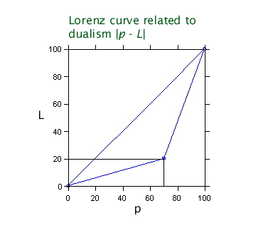
How is Dualism Measured?
One measure of dualism is simply a special case of the Gini coefficient,
in which the number of IRUs is reduced to 2. Then the Gini coefficient
can be calculated as
D = |p - L|
where p is the percentage of IRUs in the poorest category and L
is the percent income share of IRUs in the poorest category. The
symbol | | denotes the absolute value.
The relationship of dualism to the Lorenz curve and the Gini coefficient
is shown in the following exhibit.
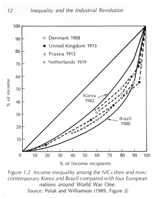
Historically the concept of dualism was emphasized in a famous article
by economist Simon Kuznets (1955) that initiated a stream of research on
the relationship of income inequality with economic development.
Kuznets thought that dualism generated by income differences between traditional/agricultural
and modern/urban sectors was a principal reason for the high level of income
inequality in developing countries. The following exhibit shows sector
dualism figures for countries of the world around 1970.
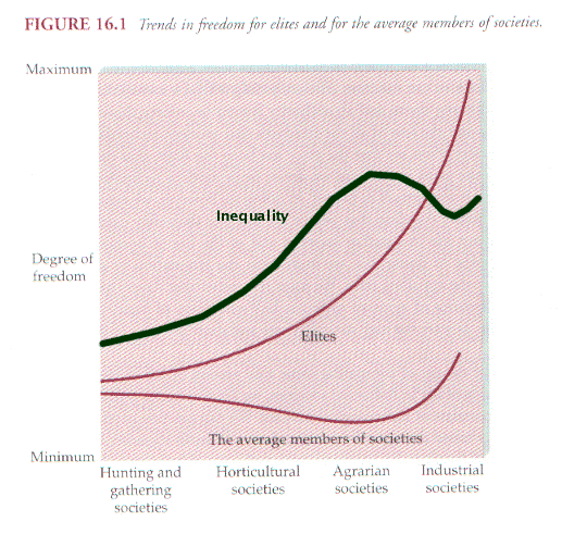
The Big Picture: Inequality Trends and Sociocultural Evolution
Is U.S. society today more or less unequal than it was 200 years ago?
How do modern industrial societies compare with simple societies, such
as hunters and gatherers?
Sociologist Gerhard Lenski has proposed a typology of human societies
based on subsistence technology, and the nature of the environment of the
society. The basic typology (simplified) is
Simplified Typology of Human Societies after Gerhard Lenski
(Nolan and Lenski 1999)
| Type of Society |
Main Technological Innovation |
Approximate Date of Appearance |
| Hunting & Gathering |
|
(primordial) |
| Horticultural |
Plant Cultivation |
8,000 BC |
| Agrarian |
Use of the Plow |
3,000 BC |
| Industrial |
Use of Machines Powered by Inanimate Forms of Energy |
1,750 AD |
Inequality has evolved in a systematic way during sociocultural evolution
according to Lenski.
Patterns of Inequality in the Modern World
During industrialization, inequality of the distribution of income has
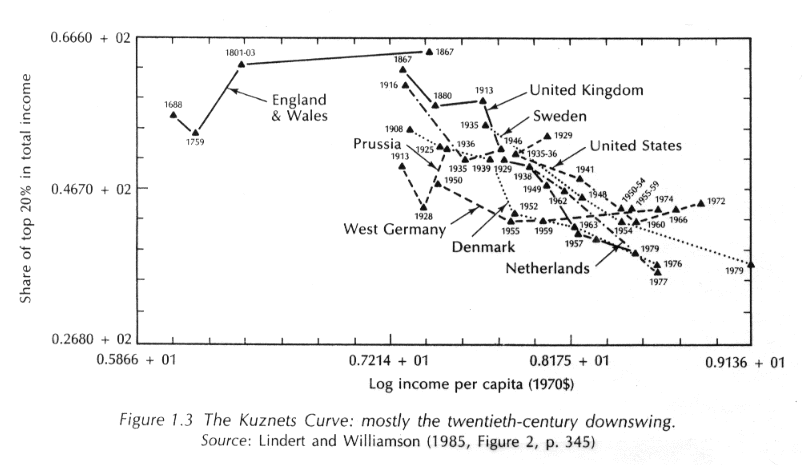
been characterized by 2 historical trends: the Kuznets Curve
and the Great U-Turn.
1. The Kuznets Curve
The Kuznets Curve was named after economist Simon Kuznets (1955).
Kuznets conjectured that during industrial development in the long run,
income inequality at first rises and then declines, tracing an inverted-U-shaped
trajectory. As a result, industrial societies are more equal than
non-industrial societies
The inverted-U shape of the Kuznets curve is due to
-
the expansion of education (producing a linear decline in inequality with
economic development)
-
the shift from agriculture to the secondary (manufacturing) and tertiary
(services) sectors (producing an inverted-U trend of inequality because
of sector dualism)
-
the demographic transition (also producing an inverted-U trend of inequality,
with inequality highest at point of fastest population growth)
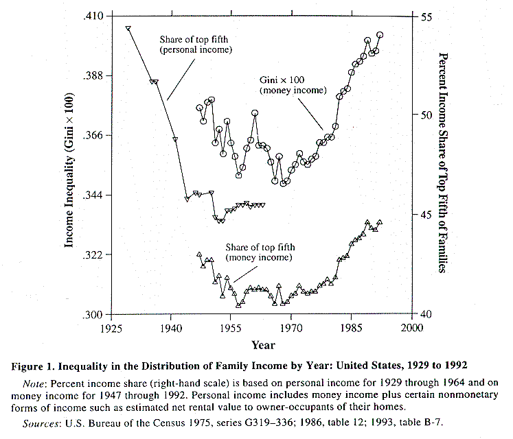
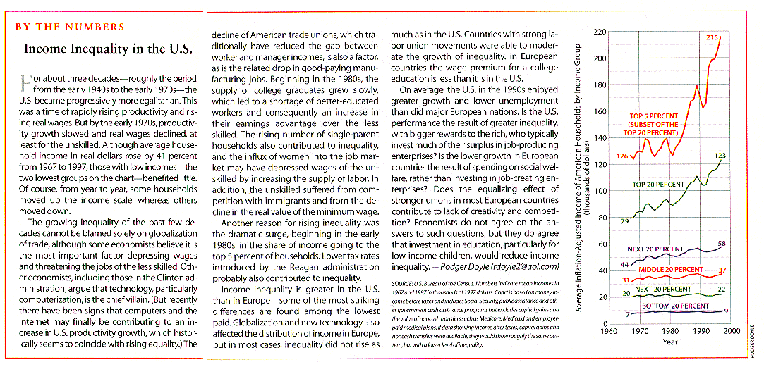
2. The Great U-Turn in the U.S. and a Few Advanced Industrial Societies
The phrase "The Great U-Turn" was coined by Harrison & Bluestone (1988).
The term refers to the inequality upswing that took place since the
early 1970s in some advanced industrial societies (especially the U.S.
and the U.K.)
Why these inequality trends?
Research suggests that the inequality upswing is the result of a combination
of factors including
-
deindustrialization ( = decline in manufacturing employment) caused in
part by globalization and international competition
-
increasing reliance on technology causing increased demand (and higher
returns) for education and cognitive skills
-
increasing proportion of female-headed households
Additional reference: the following article from the Census Bureau looks
at income inequality trends in the US from 1947 to 1998.
Two salient features of the recent trend discussed in the article are
-
in 1993 the Census Bureau changed data collection procedures of the Current
Population Survey to raise the maximum value of reported income.
This change resulted in higher inequality figures; inequality figures before
and after 1993 are therefore not comparable.
-
since 1993, inequality has not changed much (it has neither increased nor
decreased substantally)
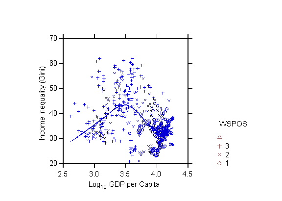
3. Current World Trends
Hans Rosling's
Gapminder site provides graphic depictions of trends in income inequality in
countries of the world.
Major trends:
- Inequality within developing countries is increasing
- Overall world inequality is decreasing because of economic
development, especially of very large countries (China, India)
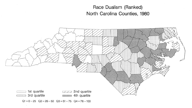
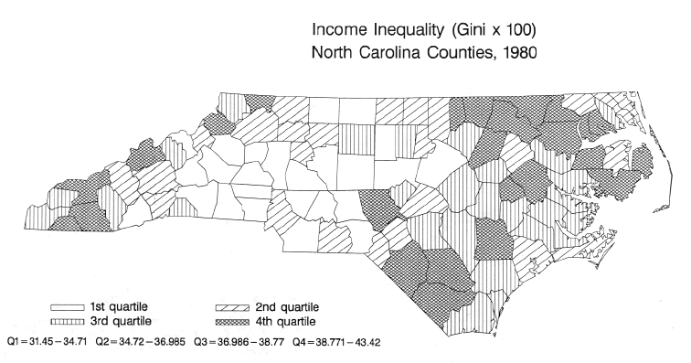
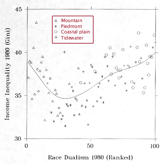
4. Regional Inequality Patterns in North Carolina
Race dualism (= inequality associated with the average income difference
between black and white families) varies among counties of North carolina.
The following exhibits show the geographical distribution at the county
level of race dualism, overall income inequality (distribution of family
income), and the relationship between income inequality and dualism.
It appears that regions of North Carolina are characterized by distinct
patterns of inequality.
Regional Inequality Patterns in North Carolina
| Region |
Race dualism |
Income inequality |
| Mountain |
Low |
High |
| Piedmont |
Low to High |
Low to High |
| Coastal plain |
High |
High |
| Tidewater |
High |
High |
Discussion: Is Bill Gates Hazardous to Your Health?
How does the degree of inequality in the social environment affect individuals
in that environment? There are many issues involved here, including
-
How can we distinguish an effect of inequality per se from the "absolute"
effects of environmental characteristics, such as hunger or poverty?
E.g.,
-
is the young man moved to break into the rich mansion because he is poor
in absolute terms, or because he cannot stand the contrast between the
luxurious lifestyle of the rich and his own modest circumstances?
-
am I depressed because I have no money, or is my depression aggravated
because I know Bill Gates has too much of it?
-
It is possible that humans are so preoccupied with issues of inequality
because evolution has given us a built-in "module" concerned with distributive
justice, as evolutionary psychologists would argue (Trivers 1971, 1985:
Chapter 15)
-
Other important concepts are related to inequality but do not coincide
with it, including
-
poverty (measured as % below a given threshold of income)
-
living standards (corresponding to some notion of average income)
-
human rights (are individuals protected from torture, loss of life,
loss of freedom at the hands of the powerful?)
-
Is there a trade-off between inequality and economic development?
One study of the effect of income inequality on health
outcomes at the county level finds a "modest independent effect [of
income inequality] on the level of depressive symptoms, and on baseline and
follow-up self-rated health, but no independent effect on biomedical morbidity
or subsequent mortality"; these effects are substantially
smaller than the effects of individual income.
References
-
Allison, Paul D. 1978. "Measures of Inequality." American
Sociological Review 43:865-80.
-
Harrison, Bennett and Barry Bluestone. 1988. The Great U-Turn:
Corporate Restructuring and the Polarizing of America. New York:
Basic Books.
-
Kerbo, Harold R. 2000. Social Stratification and Inequality.
New York: McGraw-Hill.
-
Kuznets, Simon. 1955. "Economic Growth and Income Inequality."
American Economic Review 45:1-28
-
Lecaillon, Jacques, Felix Paukert, Christian Morrisson, and Dimitri Germidis.
1984. Income Distribution and Economic Development: An Analytical
Survey. Geneva, Switzerland: International Labour Office.
-
Lindert, Peter H. 2000. "Three Centuries of Inequality in Britain
and America." Pp. 167-216 in Handbook of Income Distribution,
Volume 1, edited by Anthony B. Atkinson and François Bourguignon.
Amsterdam, Netherlands: Elsevier Science.
-
Nielsen, François. 1994. "Income Inequality & Industrial Development:
Dualism Revisited." American Sociological Review 59:654-677.
-
Nielsen, François and Arthur S. Alderson. 1997. "The Kuznets Curve
and the Great U-Turn: Income Inequality in U.S. Counties, 1970 to 1990."
American
Sociological Review 62:12-33.
-
Nielsen, François and Arthur S. Alderson. 2001. "Trends
in Income Inequality in the United States." Pp. 355-385 in Sourcebook
on Labor Markets: Evolving Structures and Processes, edited by Ivar
Berg and Arne L. Kalleberg. New York: Plenum.
-
Nielsen, François and Charles S. Warren. 1998. "Patterns of Income
Inequality in North Carolina, 1980." Sociological Analysis
1(3):87-112.
-
Nolan, Patrick and Gerhard Lenski. 1999. Human Societies:
An Introduction to Macrosociology. (8th edition.) New
York: McGraw-Hill.
-
Nygård, Fredrik and Arne Sandström. 1981. Measuring
Income Inequality. Stockholm, Sweden: Almquist and Wiskell.
-
Trivers, Robert L. 1971. "The Evolution of Reciprocal Altruism."
Quarterly Review of Biology 46:35-57.
-
Trivers, Robert L. 1985. Social Evolution. Menlo
Park, CA: Benjamin / Cummings.
Last modified 21 Feb 2008