Soci709 (formerly 209) Module 13 - THE BOOTSTRAP
Resources: ALSM5e pp. 458-464; ALSM4e pp. 429-434
1. PRINCIPLE OF THE BOOTSTRAP
The bootstrap is a computer-intensive method developed
by Bradley Efron and others to derive standard errors of estimate from
information in the sample and do statistical inference (hypothesis tests
and confidence intervals) even in nonstandard estimation situations when
there is no known analytical method to do so.
The scope of the bootrap is much broader than
linear regression models. The bootrap has been used to do statistical
inference with
-
hypothetical descent trees estimated from genetic
similarities among populations (e.g., L. Cavalli-Sforza and colleagues)
-
estimation of contour lines representing equal
altitude (or equal values of other variables) in producing maps
-
estimation of standard error of an interaction
term in models involving latent variables, etc.
Efron's standard illustration of the bootstrap
is the calculation of a standard error of estimate for the correlation
of average GPA with average LSAT scores of applicants for a sample of 15
U.S. law schools (out of a total population of 82). The following
exhibits are taken from a Scientific American article by Diaconis
& Efron (1983; see also Efron & Tibshirani 1986, 1993).
The next exhibit illustrates the concept of
sampling variation in estimating the correlation with n=15.
Exhibit:
Sampling variation of r with n=15 (Diaconis & Efron 1983 p. 122)
The original sample of 15 schools is shown.
Exhibit:
Scatterplot of average GPA against average LSAT score (Diaconis & Efron
1983 p. 118)
The principle of the bootstrap is to select a
large number of samples of size n with replacement from the original
sample. The samples are called bootstrap samples. Some cases
are typically represented more than once in a bootstrap sample.
Exhibit:
Principle of the bootstrap (Diaconis & Efron 1983 p. 119)
The standard error of estimate of the parameter
(here the correlation) is derived from the observed frequency distribution
of the estimates in the bootstrap samples (the bootstrap distribution).
Exhibit:
Frequency distribution of r with 1,000 bootstrap samples (Diaconis &
Efron 1983 p. 120)
The bootstrap distribution can be shown to be
a highly accurate approximation of the true sampling distribution of the
estimator.
Exhibit:
Comparison of bootstrap distribution of r with true distribution &
with analytically derived distribution (Diaconis & Efron 1983 p. 123)
2. THE BOOTSTRAP IN REGRESSION ANALYSIS
1. Fixed X versus Random X Sampling
In the regression context, bootstrap sampling
is done in two different ways:
-
fixed X sampling when the Xk are considered
fixed (as in experimental studies)
-
random X when the Xk are considered
random (as in observational studies).
2. Fixed X Sampling
Fixed X sampling can be used when
-
the Xk are viewed as fixed; EX: in
an agricultural experiment Y is corn yield; X1 is fertilizing
level set at 10, 20, and 30 units; X2 is watering level set
at 50, 100, 150; there are 3 plots for each fertilizer x watering
combination (n=27)
-
the regression function is a good model for the
data
-
the ei have constant variance
The fixed X sampling procedure is
-
fit the original regression
-
calculate the ei
-
sample e1*, e2*, ..., en*
from the ei with replacement and "reconstitute" observations
as Yi* = ^Yi + ei* for each original ^Yi
(i = 1, ..., n)
-
regress Yi* on the original Xi
(corresponding to that ^Yi), obtaining b*
-
do 3. to 4. "many times" (see below)
3. Random X Sampling
The random X sampling procedure can be
used when
-
the Xk are viewed as random, as in
observational studies
-
there are doubts about the adequacy of the regression
function
-
the variance of the ei is not constant
The random X sampling procedure is
-
fit the original regression, obtaining b
-
sample n cases from the original sample with
replacement, obtaining n sets (X*, Y*)
-
regress Y* on X*, obtaining b*
-
repeat 2. to 3. "many times" (see below)
The bootstrap distribution (distribution of estimates
obtained by bootstrap) for a regression coefficient looks like the following
exhibit:
Exhibit:
Bootstrapping with random X sampling (NKNW Table 10.8 & Figure
10.9 p. 433)
4. How Many is "Many Times"?
Depending on problem and the method of estimating
s*{bk*}:
-
to calculate s*{bk*} from teh bootstrap
distribution, from 50 to 200 is sufficient
-
to use the percentile method, 1,000 or more may
be needed (as the calculation of s*{bk*} depends on the tails
of the bootstrap distribution)
-
in some situations it is possible to recalculate
s*{bk*} as number of bootstrap samples increases and stop adding
samples when s*{bk*} stabilizes
3. COMPUTING s*{bk*}
FROM THE BOOTSTRAP DISTRIBUTION
1. Normal Approximation (a.k.a. Naive Bootstrap)
Calculate s*{bk*} as the standard deviation
of the bk*. Then calculate a CI for bk
assuming that the sampling distribution of bk is normal, as
CI{bk} = (bk(obs)
- t(1-a/2, k-1)s*{bk*},
bk(obs) + t(1-a/2,
k-1)s*{bk*})
where bk(obs) is the estimate of the
regression coefficient from the original sample, k is the number of bootstrap
samples, and t(1-a/2,
k-1) is the 100(1-a/2)
percentile of the Student t distribution with k-1 df. (For reasons
that are not yet entirely clear to me this method is sometimes called "naive".)
Another quantity associated with this approach
is the estimated bias, which is calculated as bk(obs)
minus the mean of the bootstrap estimates of bk.
2. Percentile Method
The CI for bk is estimated by the percentile
method as
(bk* (a/2),
bk*(1-a/2))
where bk*(p) is the 100pth percentile
of the empirical bootstrap distribution. So for example the 95 percent
CI is bound by the 2.5th and 97.5th percentiles of the bootstrap distribution.
The percentile method requires at least 500 bootstrap samples because the
method uses the tails of the bootstrap distribution.
(ALSM5e and ALSM4e discuss a variant of the
percentile method called the reflection method that I do not fully
understand.)
3. Other Methods
STATA offers two additional methods for estimating
the CI called the bias-corrected method and the bias-corrected
and accelerated method. Sounds irresistible.
See STATA documentation for command [R] bootstrap.
4. EXAMPLES
1. Spearman Rank Correlation for Efron's
Law School Data (SYSTAT)
This example is from SYSTAT V7 New Statistics
pp. 8-9.
This replicates Diaconis and Efron's (1983)
analysis but for the Spearman rank correlation rather than the Pearson
correlation; 1,000 bootstrap samples are produced.
Exhibit:
Scatterplot of GPA by LSAT - original sample (n=15)
m13008.gif (alternate picture)
Exhibit: Bootstrap
analysis of Spearman rank correlation of GPA with LSAT (1,000 samples)
Exhibit: Bootstrap
analysis of Spearman rank correlation of GPA with LSAT- program only
Exhibit: Frequency
distribution of bootstrap estimates (n=1,000)
m13011.gif (alternate picture)
2. Linear Regression Model with the Longley
Data (SYSTAT)
This example is provided with the SYSTAT 9 help
system.
Exhibit:
Bootstrap analysis of the Longley data
3. Robust Estimation of Yule Model Using
Bisquare Formula (SYSTAT)
(The following example uses a syntax to save teh
bootstrap estimates that was originally undocumented.)
Exhibit:
Bootstrap analysis of Yule's model with OLS and robust regression (bisquare
3.5)
Exhibit: Same
- program only (yuleboot.syc)
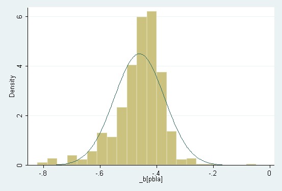
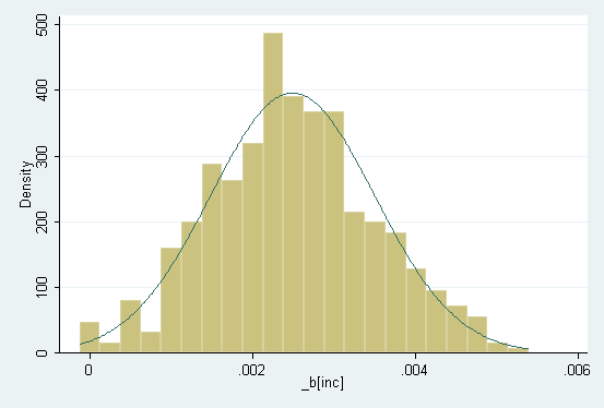
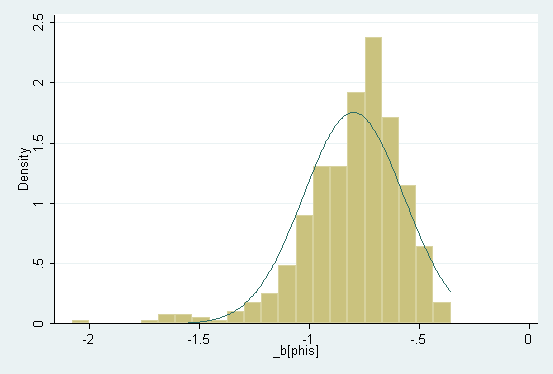
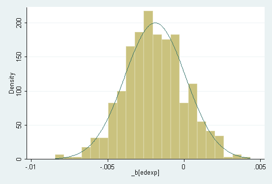
4. Robust Estimation of the Graduation Rate Model (STATA)
Exhibit: Bootstrap analysis of robust
regression of graduation rate model
Exhibit: Bootstrap distribution of b_pbla
(histogram)
Exhibit: Bootstrap distribution of b_inc
(histogram)
Exhibit: Bootstrap distribution of b_phis
(histogram)
Exhibit: Bootstrap distribution of b_edexp
(histogram)
Last modified 17 Apr 2006