SOCI209 - Module 2 - INFERENCE IN SIMPLE LINEAR REGRESSION
1. Inference in Regression Models
From Module 1 the parameters b1 and
b0 are estimated as
b1 = (S(Xi
-
X.)(Yi - Y.))/S(Xi
-
X.)2
b0 = Y.-
b1X.
Just like other statistics (such as the sample mean or variance) the estimates
b1 and b0 are functions of the observed values Yi,
which are functions of the random errors ei.
Thus b1 and b0 are themselves random variables and
b1 and b0 each has a probability distribution, called
the sampling distribution. The sampling distribution of b1
(respectively b0) refers to "the different values of b1
(b0) that would be obtained with repeated sampling when the
levels of the independent variables X are held constant from sample to
sample" (ALSM5e p. 41; ALSM4e p. 45). Statistical inference
concerning populations parameters such as b1
and b0 consists in testing hypotheses
and constructing confidence intervals for that parameter. Inference
concerning a parameter is based on the sampling distribution of that parameter.
For (simple or multiple) linear regression models statistical inference
is commonly carried out for
-
the regression coefficients b1
and b0 (hypothesis tests and confidence
intervals)
-
the mean response E{Yh} knowing Xh (whether Xh
corresponds or not to an observation in the sample) (confidence intervals
only)
-
the individual value of a "new" observation Yh(new) knowing
Xh (whether Xh corresponds or not to an observation
in the sample) (confidence intervals only)
-
F test of the significance of the regression model as a whole (test only)
2. Inference on b1 and
b0
1. Sampling Distribution of b1
The informal derivation below shows that if the errors ei
are normally distributed the sampling distribution of t*=(b1-
b1)/s{b1} is a Student
t distribution with (n-2) degrees of freedom (df). t* refers to the
deviation (b1- b1) of
b1 from its expectation (b1)
divided by the estimated standard error s{b1} of b1
(i.e., the estimated standard deviation of the sampling distribution of
b1). The standard error s{b1} is estimated
from the data as s{b1}=[MSE/S(Xi
- X.)2 ]1/2. Thus t is the standardized
value of b1 (i.e., a z-score). When the distribution of
errors is not too far from normal and the sample is not too small the distribution
of t
approximately follows a Student t distribution. Even
when the distribution of errors is far from normal, the distribution of
t* approaches a Student t distribution (actually a normal distribution)
as the sample size n becomes large.
Informal derivation of the sampling distribution of t*
|
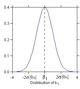
STEP 1: Sampling Distribution of b1
Assuming that errors are normally distributed
b1 ~ N ( b1
, s2{b1})
(~ means is distributed as)
where s2
denotes the variance of ei and s2{b1}
= s2
/ S(Xi - X.)2.
In words: b1 is normally distributed with mean E{b1}
= b1 and variance s2{b1}
= s2
/ S(Xi - X.)2
(figure at left).
The sampling distribution of b1 is normal because b1
is a linear combination of the observations Yi which are independent
normally distributed random variables (ALSM5e, ALSM5e: Appendix A, Theorem
A.40). Note the denominator S(Xi
- X.)2 in the expression for s2{b1}:
the greater the variance of X, the smaller the variance
s2{b1}
of the sampling distribution, and the more precise the estimation of b1.
(In experimental research, where the experimenter sets the values of X,
one may be able to space the X values optimally to achieve the smallest
s2{b1}
possible.) |
 Distribution of (b1-b1)/
s{b1}
Distribution of (b1-b1)/
s{b1}
|
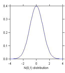
STEP 2: Distribution of (b1-b1)/s{b1}
(b1-b1)/s{b1}
~ N (0, 1)
In words: the deviation of b1 from its mean b1
, divided by the standard error
s{b1},
is normally distributed with mean 0 and standard deviation 1 (i.e., according
to a standard normal distribution). This follows from STEP 1 by applying
to b1 by the equivalent of the z transformation z = (X - m)/s.
s{b1} denotes the standard deviation
of the sampling distribution of b1. s{b1}
is called the standard error of b1. |
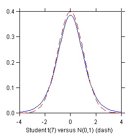 Distribution of t* = (b1- b1)/
s{b1} (solid
Distribution of t* = (b1- b1)/
s{b1} (solid
blue line) compared to distribution of
(b1- b1)/
s{b1}
(red dashed line)
|
STEP 3: Distribution of (b1 - b1)/
s{b1}
In practice
s{b1} is not known (because
s is not known) so one replaces the standard
error
s{b1} with the sample estimate
s{b1} given by
s{b1} = [MSE / S(Xi
- X.)2]1/2
where MSE is the mean squares error. When s{b1}
is replaced by the sample estimate s{b1}, the sampling distribution
is no longer normal. It becomes a Student t distribution with (n-2)
df:
t* = (b1- b1)/
s{b1} ~ t (n - 2)
The distribution is no longer normal because s{b1} (being a
sample estimate) is a random variable rather than a fixed constant. This
"extra randomness" produces the thicker tails of the t distribution
compared to the normal. The (n - 2) df correspond to the (n - 2)
df of MSE (see Module 1).
|
The derivation of the sampling distribution of b0 is shown later.
Inference on the regression coefficients uses the following formulas.
Table 1. Formulas for Inference on b1 and
b0
| Slope b1 |
|
| Estimated standard error of b1 |
s{b1} = (MSE/S(Xi
- X.)2)1/2 |
| Estimated sampling distribution of b1 |
(b1 - b1)/s{b1}
~ t(n - 2) |
| Confidence limits for CI on b1 |
b1 +/- t(1 - a/2; n - 2)s{b1} |
| Test statistic for H0: b1
= b10 |
t* = (b1 - b10)/s{b1}
(1) |
| Intercept b0 |
|
| Estimated standard error of b0 |
s{b0} = (MSE(1/n+X.2/S(Xi
- X.)2)1/2 |
| Estimated sampling distribution of b0 |
(b0 - b0)/s{b0}
~ t(n - 2) |
| Confidence limits for b1 |
b0 +/- t(1 - a/2; n - 2)s{b0} |
| Test statistic for H0: b0
= b00 |
t* = (b0 - b00)/s{b0}
(1) |
Notes: (1)
-
b10 and b00
denote hypothetical values of the parameters
-
when b10 = 0 (the most
common type of hypothesis) then t* = b1/s{b1}
|
The estimated standard error s{b1} is typically provided
in the standard regression printout (labeled Std Error in Table 2).
Table 2 repeats the regression printout used for illustration.
Table 2. Printout of Regression of % Clerks on Seasonality
Index
Dep Var: CLERKS
N: 9 Multiple R: 0.852 Squared multiple R: 0.726
Adjusted squared multiple
R: 0.687 Standard error of estimate: 2.103
Effect
Coefficient Std Error Std Coef
Tolerance t P(2 Tail)
CONSTANT
14.631 1.700
0.000 .
8.607 0.000
SEASON
-0.169 0.039
-0.852 1.000 -4.311
0.004
Analysis of Variance
Source
Sum-of-Squares df Mean-Square
F-ratio P
Regression
82.199 1 82.199
18.583 0.004
Residual
30.963 7
4.423
2. Inference on b1
We look at inference on b1 first
because it is the most common.
Confidence Interval for b1
From Table 1 the confidence limits of the CI for b1
are
b1 +/- t(1 - a/2; n -
2)s{b1}
where t(1 - a/2; n - 2) refers to the (1 - a/2)100th
percentile of the Student t distribution with (n-2) df.
Example: find the 95% CI for b1,
the coefficient of seasonality in the simple regression of % clerks.
b1 = -.169 (from regression printout under Coefficient)
s{b1} = .039 (from regression printout under Std Error)
choose a = .05; then t(1-a/2;
n-2) = t(.975; 7) = 2.365 (from statistical program or from table)
Therefore the 95% CI for b1 is
L = -.169 - (2.365)(.039) = -0.261 (lower bound of CI)
U = -.169 + (2.365)(.039) = -0.077 (upper bound of CI)
One can say that with 95% confidence
-0.261 <= b1 <=
-0.077
Two-sided test for b1
Example: Test the hypothesis that the coefficient of seasonality b1
= 0. The setup is
H0: b1 = 0
("null hypothesis")
H1: b1<>
0 ("research hypothesis")
The test statistic corresponding to H0: b1
= 0 is
t* = (b1 - 0)/s{b1} = b1/s{b1}
(provided in the regression printout under t).
Choose a significance level a = .05.
Using the P-value approach, the test statistic is
t* = (-.169)/(.039) = -4.311 (also from regression printout
under t)
Find the 2-tailed P-value
P{|t(n - 2)| > |t*| = 4.311 = .004 (from regression printout
under P(2 Tail)).
Since P-value = .004 < a = .05, one concludes
H1, that "there is a significant linear association between
% clerks and seasonality", or "the coefficient of seasonality is significant
at the .05 level". (One would actually say "at the .01 level" in
this case, choosing the lowest "round" significance level greater than
the P-value .004.)
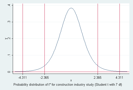
Using the decision theory method the decision rule is
if |t*| <= t(1-a/2; n-2), conclude
H0
if |t*| > t(1-a/2; n-2), conclude H1
With a = .05, t(1-a/2;
n-2) is
t (0.975; 7) = 2.365
Since |t*| = 4.311 > 2.365 conclude H1 (b1<>
0) at the .05 level with this method also.
One-sided test for b1
Hint: It is often easier to write down H1 (the "research hypothesis")
first; then H0 is the complement of H1
In the regression of % clerks on seasonality the one-sided test is
lower-tailed, since b1 (-.169) is negative, so the hypothesis
setup is
To carry out the test
-
if b1 is in a direction opposite to H1 (i.e., if
b1 > 0), then there is no point in doing the test
and H1 can be rejected at the outset
-
otherwise (b1 is in a direction compatible with H1)
using the P-value approach one simply calculates the 1-sided P-value associated
with b1 by dividing the 2-tailed P-value (shown on the regression
printout) by 2
In the example the 2-sided P-value is .004; thus the 1-sided P-value is
P(t(n - 2) < t*) = (.004)/2 = .002
Since P-value = .002 < .05 = a, conclude
H1: b1
< 0.
Using the decision theory method the decision rule is
if |t*| <= t(1-a; n-2), conclude
H0
if |t*| > t(1-a; n-2), conclude H1
In the example
t(1-a; n-2) = t(0.95; 7) = 1.895
Since |-4.311| > 1.895, conclude H1: b1
<
0 by this method also.
Comparing Two-sided and One-sided Tests for b1
Comparing the two types of tests it appears that the 1-sided test is
"easier" (i.e., more likely to turn up significant) than the corresponding
2-sided test. (For example, the P-value of the 1-sided test is
half the P-value of the 2-sided test.)
Thus there is an incentive to use 1-sided tests to increase the chance
of significant results. It is considered legitimate to use a 1-sided
test whenever one has a genuine directional hypothesis concerning b1.
In the construction industry study the author's expectation that greater
seasonality is associated with less bureaucracy (implying a negative slope)
is a genuine directional hypothesis. Thus a 1-sided test is appropriate
in this case. (In any case in this example the slope is significant
in the 2-sided test, too.) This opinion on the use of one-tailed
tests is widely shared by reviewers of professional journals. However,
some statisticians recommend using 2-sided tests exclusively, on the ground
that the 2-sided test is conservative.
3. Inference on b0
CIs and tests for b0 are carried
out in exactly the same way as for b1.
Q - Using information from the printout
-
calculate the 95% CI for b0
-
test the 2-sided hypothesis that b0
<> 0
4. (Optional) Sampling Distribution of b0
The intercept b0 is estimated as
b0 = Y. - b1X.
The estimated standard error of b0 is
s{b0} = (MSE(1/n+X.2/S(Xi
- X.)2)1/2
The standardized statistic
t* = (b0 - b0)/s{b0}
is distributed as t(n - 2)
(See ALSM5e pp. 48-49; ALSM4e pp. <>)
3. Inference for Mean Response E{Yh}
1. Sampling Distribution of ^Yh
The mean response E{Yh} is estimated as ^Yh
= b0 + b1Xh. Thus the variance of
the sampling distribution of ^Yh is affected by variance in
both b0 and b1 sampling and by how far Xh
is from the sample mean of X. The way in which the variance of ^Yh
depends on the distance of Xh from X. is shown in
the next exhibit: given a change in b1, the change in ^Yh
is larger further away from the mean.
Table 3. Formulas for Inference on ^Yh
| Point estimator of E{Yh} |
^Yh = b0 + b1Xh |
| Estimated standard error of ^Yh |
s{^Yh} = (MSE ((1/n) + (Xh - X.)2
/ S(Xi - X.)2))1/2 |
| Estimated distribution of ^Yh |
(^Yh - E{Yh}) / s{^Yh} ~ t (n-2) |
| Confidence limits for CI on E{Yh} |
^Yh +/- t(1- a/2; n-2)s{^Yh} |
| Test statistic |
Not often used |
Notes:
-
Xh is a given level of X which does not necessarily correspond
to a data point Xi
-
the standard error of ^Yh is affected by (Q - explain how)
-
MSE
-
(Xh - X.) the deviation of Xh from the
sample mean of Xi
-
variability of Xi
-
sample size n
|
2. CI for Mean Response E{Yh}
Example 1
Given the regression of % clerks on seasonality, calculate an interval
estimate for E{Yh} when seasonality is 35, i.e. Xh
= 35.
First calculate s{^Yh}.
From the regression printout in Table 2 n = 9 and MSE = 4.423.
One needs additional information not contained in the standard regression
output.
From Module 1, Table 1: X. = 39.556; S(Xi
- X.)2 = 2886.222.
For Xh = 35, ^Yh = 14.631 + (-0.169)(35) = 8.716
and (Xh - X.)2 = (35 - 39.556)2
= 20.757.
Thus s{^Yh} = (4.423((1/9) + 20.757/2886.222))1/2
= 0.7233628.
Choose a = .05, so that t(.975;7) = 2.365.
Then the confidence limits for E{Yh} are
L = 8.716 - (2.365)(0.7233628) = 7.005 (lower bound)
U = 8.716 + (2.365)(0.7233628) = 10.427 (upper bound)
so that with 95% confidence
7.005 <= E{Yh|Xh = 35} <= 10.427
Example 2
This example illustrates a technique to obtain s{^Yh} from the
computer rather than computing it "by hand".
The example uses the data set knnappenc07.syd (see KNN Appendix
C data set 07). Units are 522 home sales in a mid-western town.
Y is the sale price in dollars; X is the finished area of the home in square
feet. The county tax collector runs a simple regression of sale price
on finished area, obtaining
^Y = -81432.9464 + 158.9502X n=522 R2
= .6715
The tax collector wants to estimate of the average sale price (i.e.,
E{Yh}) of homes with 2,500 square feet of finished area and
obtain a 95% CI for that average sale price. To calculate both ^Yh
and s{^Yh} quickly, the tax collector adds a 523d "dummy" case
to the data set, with only the value of 2500 for X and missing value for
Y and re-runs the regression. Then he obtains ^Yh
and s{^Yh} for all observations, including the dummy one (STATA
predict yhat, xb; predict seyhat, <>; SYSTAT save resid
with variables ESTIMATE and SEPRED).
So for Xh=2500
^Yh = 315942.6306
s{^Yh} = 3654.4390
Thus using the formula above the 95% CI for the average sale price
of homes with 2,500 square feet of finished space is
L = 315942.6306 - (1.9645365)(3654.4390) = 308763.35
(lower bound)
U = 315942.6306 + (1.9645365)(3654.4390) = 323121.91 (upper bound)
Note that this is a relatively narrow interval, indicating that the average
sale price of 2500 square feet homes can be estimated quite precisely.
3. CI for the Entire Regression Line - the Working-Hotelling Confidence
Band
The Working-Hotelling confidence band is a CI for the entire regression
line E{Y} = b0+b1X.
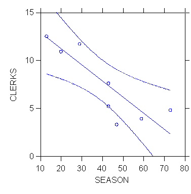
The next exhibit shows the 95% Working-Hotelling confidence band for the
regression of % clerks on seasonality. The W-H confidence band is
often examined graphically.
The bounds of the (1-a) W-H confidence band
for Xh are given by
^Yh +/- Ws{^Yh}
where
W = [2F(1-?; 2, n-2)]1/2
(See ALSM5e pp. 61-63.)
4. (Optional) Derivation of Sampling Distribution of ^Yh
The standard error of ^Yh is estimated as
s{^Yh} = (MSE ((1/n) + (Xh - X.)2
/ S(Xi - X.)2))1/2
(^Yh - E{Yh})/s{^Yh} is distributed as
a t distribution with (n-2) df. (See ALSM5e pp. 52-54.)
4. Prediction Interval for a New Observation Yh(new)
1. Sampling Distribution of Yh(new)
Prediction intervals are especially important for quality control
(QC) in an industrial context. (The procedure is explained in detail
in ALSM5e pp. 55-61; ALSM4e pp. 61-66 pp. 61-66.)
Examples:
-
predict first-year college GPA of an individual student (not in the sample),
knowing his/her SAT and the regression of GPA on SAT
-
predict the sale price of an individual home that has 2500 square feet
of finished space, in a certain Midwestern town
In both cases one is trying to predict the value Yh(new) of
the response for an individual case with a specific value Xh
of the independent variable. This is different from the previous
situation where one wants to estimate the average value of Y for
X=Xh.
One estimates Yh(new) as ^Yh,= b0+b1Xh,
the value of ^Y on the regression line corresponding to Xh.
Variation in Yh(new) is affected by two sources:
-
variation in ^Yh, the estimated mean of the distribution of
Y given Xh, namely s2{^Yh}
-
variation in the probability distribution of Y around its mean given Xh,
namely s2
The decomposition of the variation in Yh(new) is shown in the
next two exhibits.
Therefore,
s2{Yh(new)}
= s2
+ s2{^Yh}
Thus the sampling disribution of Yh(new) is described as in
the following table.
Table 4. Formulas for Inference on Yh(new)
| Point estimator of Yh(new) |
^Yh = b0 + b1Xh |
| Estimated standard error s{Yh(new)} (s{pred}) |
s{pred} = (MSE (1 + (1/n) + (Xh - X.)2
/
S(Xi - X.)2
))1/2 |
| Estimated distribution of Yh(new) |
(Yh(new) - E{Yh}) / s{pred} ~ t (n-2) |
| Confidence limits for CI on Yh(new) |
^Yh +/- t(1- a/2; n-2)s{pred} |
| Test statistic |
Not often used |
2. CI for Yh(new)
This example uses again the SYSTAT data set knnappenc07.syd (see
KNN Appendix C data set 07). Units are 522 home sales in a mid-western
town. Y is the sale price in dollars; X is the finished area of the
home in square feet. The estimated regression is
^Y = -81432.9464 + 158.9502X n=522 R2
= .6715
Imagine this time that that someone plans to sell their home in this Midwestern
town. They ask a real-estate agent to estimate the price the home
might fetch on the market, given that it has 2500 square feet of finishes
space, and to give them a 95% CI for that price. The real estate
agent uses the same trick as the tax collector, of adding a "dummy" 523d
case with X = 2500 to obtain both ^Yh and s{^Yh};
she also obtains MSE from the regression printout, so she has the following
information
^Yh = 315942.6306
s{^Yh} = 3654.4390
MSE = 6.26043E+09
From this information she calculates s2{Yh(new)}
as
s2{Yh(new)}
= s2 + s2{^Yh}
= MSE + (SEPRED)2 = 6.26043E+09 + (3654.4390)2 =
6273784924.40
Hence s{Yh(new)} = (6273784924.40)1/2 = 79207.23.
Thus the 95% CI for the estimated sale price of an individual 2500
square feet home is obtained as
L = 315942.6306 - (1.9645365)(79207.23) = 160337.14 (lower
bound)
U = 315942.6306 + (1.9645365)(79207.23) = 471548.12 (upper bound)
Note that the 95% CI for Yh(new) (160K to 472K) is considerably
wider than the CI for the mean response E{Yh} (309K to 323K).
(Q - Why is that?)
3. (Optional) Derivation of Sampling Distribution of
Yh(new)
See ALSM5e pp. 55-60.
5. F Test for Entire Regression (Alternative Test of b1
= 0)
1. F Test of b1 = 0
Here this test is overkill, since the t test can be used to test the hypothesis
that b1 = 0.
But the F test generalizes to multiple regression to test the hypothesis
that all the regression coefficients are zero.
2. Expected Mean Squares
One can show that
E{MSE} = s2
E{MSR} = s2
+ b12 S(Xi
- X.)2
(ALSM5e pp. 68-71; ALSM4e pp. 75-76)
Note that if b1=0, E{MSR}
= E{MSE} = s2.
Therefore, an alternative to the 2-sided hypothesis test for b1
H0: b1 = 0
H1: b1 <> 0
is the F test
F* = MSR/MSE
If b1 = 0, E{F*} = s2/s2
= 1.
If b1<> 0, E{F*} > 1.
Thus the larger F*, the more likely that b1
<>
0.
It can be shown that if H0 holds (i.e., if b1=0)
F* = MSR/MSE ~ (c2(1)/1
) / (c2(n-2)/(n-2)) = F(1; n-2)
(ALSM5e p. 70; ALSM4e pp. 76-77)
3. Carrying Out the F Test
Example: Carry out the F test for the regression of % clerks on seasonality.
Choose a = .05.
Using the P-value method, calculate F* as
F* = MSR/MSE = (82.199)/(4.423) = 18.583
The P-value is P{F(1;7) > 18.583} = 0.004.
Since P-value = 0.004 < .05 = a, conclude
H1: b1 <> 0.
Using the decision theory method, the decision rule is
if F* <= F(1-a ; 1, n-2), conclude
H0
if F* > F(1-a ; 1, n-2), conclude H1
F(1-a ; 1, n-2) = F(0.95;1,7) = 5.59.
Since F* = 18.583 > 5.59, conclude H1: b1
<> 0 by this method also.
The principle of the decision theory method is shown in the next exhibit.
4. Equivalence of t Test and F Test
In the simple linear regression model, F* = (t*)2.
Example: In the regression of % clerks on seasonality, the squared
t-ratio for b1 is equal to F*, i.e.
(t*)2 = (-4.311)2 = 18.583 = F*
This is no longer true in the multiple regression model.
6. Maximum Likelihood Estimation
When the functional form of the probability distribution of ei
is specified (as in this case, where it is assumed normal), one can estimate
the parameters b0
, b1
and s2
by the maximum likelihood (ML) method. In essence, the ML
method "chooses as estimates those values of the parameters that are most
consistent with the sample data" (ALSM4e p. 30).
1. ML Estimation of the Mean m
Assume Y normally distributed and variance known (s
= 10); estimate mean m from sample with n =
3 (Y1 = 250, Y2 = 265, Y3 = 259).
Given an estimate of m, the likelihood L
of the sample (Y1, Y2, Y3) is the product
of the probability densities of the Yi given the value of the
estimated mean.
The normal probability density function is f(Y) = (1/(SQRT(2p)s))
exp(-(1/2)((Y- m)/s)2)
(ALSM4e Appendix A, Theorem A.34).
Example:
If m = 230, then f(Y1)
= 0.053991, f(Y2) = 0.000873, f(Y3) = 0.005953
so that
L (m = 230) = (0.053991)(0.000873)(0.005953)
= (.279)10-6
Similarly, if m = 259, then
L (m = 259) = (0.333225)(0.398942)(0.266085)
= 0.035373
Thus, the likelihood that m = 259 is greater
than the likelihood of m = 230.
(NOTE: Figures for the densities in NKNW p. 31 are incorrect;
they are all shifted 1 decimal place to the right.)
Graphically the situation is as in the next exhibit:
One could calculate the likelihood of the sample over a range of closely-spaced
values of m and graph the resulting likelihood
function of m. as in the following
exhibit:
The value of m corresponding to the maximum
of the likelihood function (here m = 258) is
the ML estimate of m. In practice
the value(s) of the parameter(s) that maximize the likelihood function
are found by iterative numerical optimization methods.
2. ML Estimation of the Normal Regression
Model
The principle for ML estimation of regression model is the same as for
m.
The likelihood function is as shown in NKNW Equation 1.26 p. 34.
The ML estimates of are the values that maximize this likelihood
function.
For teh simple regression model they are:
|
Parameter
|
ML Estimator
|
Remark
|
|
b0
|
^b0 = b0
|
same as OLS
|
|
b1
|
^b1 = b1
|
same as OLS
|
|
s2
|
^s2
= SSE/n
|
<> OLS (MSE = SSE/(n-2))
|
NOTE: maximum likelihood derivations often use the logarithm (base e)
of L rather than L itself. See NKNW Equation 1.29 p. 35.
7. Statistical Inference in Practice
1. SYSTAT Commands for Simple Regression
The following printout shows how to obtain the simple regression of % clerks
on seasonality, plot the corresponding scatterplot with the estimated regression
line and the 95% Working-Hotelling confidence band, and how to get s{^Yh}
for Xh = 35 (a value of seasonality that does not correspond
to any case in the data set) by adding a dummy case with SEASON = 35 and
missing value for CLERKS.
>USE "Z:\mydocs\S208\craft.syd"
SYSTAT Rectangular file
Z:\mydocs\S208\craft.syd,
created Thu Nov 07,
2002 at 08:24:57, contains variables:
TYPE$
SIZE SEASON
CLERKS
>regress
>rem can also use
command MGLH instead of REGRESS
>model clerks=constant+season
>estimate
Dep Var: CLERKS
N: 9 Multiple R: 0.852 Squared multiple R: 0.726
Adjusted squared multiple
R: 0.687 Standard error of estimate: 2.103
Effect
Coefficient Std Error Std Coef
Tolerance t P(2 Tail)
CONSTANT
14.631 1.700
0.000 .
8.607 0.000
SEASON
-0.169 0.039
-0.852 1.000 -4.311
0.004
Analysis of Variance
Source
Sum-of-Squares df Mean-Square
F-ratio P
Regression
82.199 1 82.199
18.583 0.004
Residual
30.963 7
4.423
-------------------------------------------------------------------------------
Durbin-Watson D Statistic
1.995
First Order Autocorrelation
-0.107
>rem show a scatterplot
with the regression line
>rem and the Working-Hotelling
95% confidence band
>plot clerks*season/stick=out
smooth=linear short confi=0.95
>rem now add a case
with Xh=35, missing Y, using menus
>rem redo the estimation
and save residuals to get SEPRED
>model clerks=constant+season
>save clerkres
>estimate
1 case(s) deleted due
to missing data.
<...repeat output
deleted...>
Residuals have been saved.
>use clerkres
SYSTAT Rectangular file
Z:\mydocs\s208\clerkres.SYD,
created Fri Nov 15,
2002 at 10:20:07, contains variables:
ESTIMATE
RESIDUAL LEVERAGE COOK
STUDENT SEPRED
>list estimate residual
sepred
Case number
ESTIMATE RESIDUAL
SEPRED
1 2.311
2.489 1.485
2 7.374
0.226 0.714
3 9.737
1.963 0.814
4 6.699
-3.399 0.759
5 7.374
-2.174 0.714
6 9.737
1.963 0.814
7 11.256
-0.356 1.038
8 12.437
0.063 1.254
9 4.674
-0.774 1.035
10 8.724
. 0.723
>rem SEPRED = 0.723
for SEASON=35 is same as calculated by hand earlier
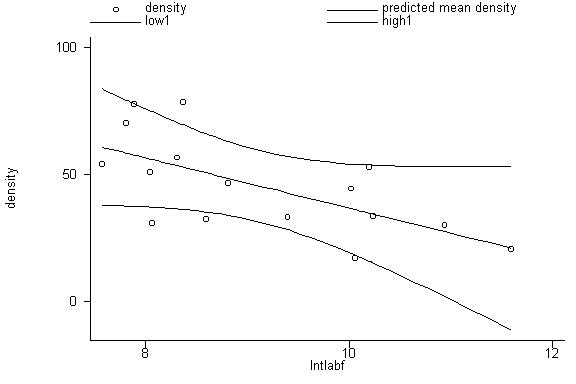
2. STATA Commands
. reg density lntlabf
Source |
SS df
MS
Number of obs = 16
---------+------------------------------
F( 1, 14) = 10.28
Model |
2260.31012 1 2260.31012
Prob > F = 0.0063
Residual | 3078.52104
14 219.89436
R-squared = 0.4234
---------+------------------------------
Adj R-squared = 0.3822
Total |
5338.83116 15 355.922077
Root MSE = 14.829
------------------------------------------------------------------------------
density |
Coef. Std. Err. t
P>|t| [95% Conf. Interval]
---------+--------------------------------------------------------------------
lntlabf |
-9.889076 3.084457 -3.206
0.006 -16.50458 -3.273573
_cons |
135.7141 28.3748 4.783
0.000 74.85625
196.572
------------------------------------------------------------------------------
. predict yhat
[option xb assumed;
fitted values]
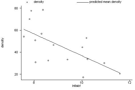
. label variable
yhat "predicted mean density"
. predict e, resid
. label variable
e "residual"
. generate yhat0=_b[_cons]
+ _b[lntlabf]*lntlabf
. generate e0=density-yhat0
. predict new, stdp
. graph density yhat
lntlabf, connect(.s) symbol (Oi) ylabel xlabel
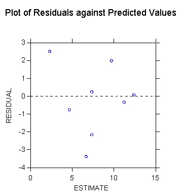
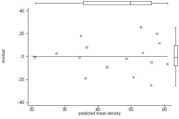
. graph e yhat, twoway
box yline(0) ylabel xlabel
. display invttail(14,.025)
2.1447867
[If you’d rather use
the F-value here, use the command invFtail (dfn,dfd, p)]
. generate low1=yhat-2.1448*new
. generate high1=yhat+2.1448*new
. graph density yhat
low1 high1 lntlabf, connect(.sss) symbol(Oiii) ylabel xlabel
10. Historical Note
1. The Normal Distribution
The discoveries of the normal probability distribution and of the central
limit theorem are associated with mathematicians Pierre Simon Laplace and
Carl Friedrich Gauss.
Q - What languages are Laplace and Gauss using in these excerpts?
Why?
2. The Student t Distribution
The Student t distribution was discovered by William Gosset.
Q - Do you know the origin of the name "Student"?
Last modified Jan 2006
![Exhibit: Working-Hotelling CI for regression of % clerks on seasonality [m16001.jpg]](m16001.jpg)
![Exhibit: Principle of F test (NWW F19.3 p. 580) [m2009.gif]](m2009.gif)