SOCI709 (formerly 209) - Module 3 - Diagnostics & Remedies in Simple
Regression
1. Residual Analysis & the Healthy Regression
1. Residual Plot of the Healthy Regression
Residual analysis is a set of diagnostic methods for investigating
the appropriateness of a regression model based on the residuals
ei = Yi - ^Yi
where ^Yi is the fitted value (aka predictor, aka estimate)
^Yi = b0 + b1Xi
The basic idea is that, if the regression model is appropriate, the residuals
ei should "reflect the properties ascribed to the model error
terms ei", such as independence,
constant variance for different levels of X and normal distribution.
The workhorse of residual analysis is the
residual plot, or plot
of the residuals ei against the fitted values
^Yi = b0 + b1Xi.
In a healthy regression the residuals should appear as arranged randomly
in a horizontal band around the Y = 0 line, like so
In reality, computer programs typically adapt the range of the data
to occupy the entire frame of the plot, so that the residuals appear as
a random cloud of points spread out over the entire vertical range of the
plot. The next exhibit shows a typical computer-generated residual
plot
2. Potential Problems With the Simple Regression Model
Problems with the regression are departures from ( or violations of)
the assumptions of the regression model. They are:
-
Regression function is not linear
-
Error terms do not have constant variance
-
Error terms are not independent
-
Model fits all but one or a few outlier observations
-
Error terms are not normally distributed
-
One or several important predictor variables have been omitted from model
These problems also affect multiple regression models. Most of the
diagnostic tools used for simple linear regression are also used with multiple
regression.
This module examines these potential problems in conjunction with diagnostic
tools which can be informal (such as graphs) or formal (such
as tests), and remedies.
3. Using Informal (Graphic) Versus Formal Diagnostic Tests
Features of informal graphic diagnostics are
-
they are visual and at least in part subjective
-
they may be inconclusive
-
they require judgment, and therefore
-
they may require training and/or experience
-
sometimes judgment may be helped by calibration (see normal probability
plot, later)
Features of formal tests are
-
they may give a straight yes/no answer about presence of a problem
-
they may not require experience or training
-
they may be used in automatic fashion
-
they may not reveal the substantive situation as well as informal tools,
so that
-
researcher relying entirely on formal tools may miss an interesting aspect
of the data (e.g., in Box-Cox estimation of optimal transformation of the
data)
Researchers can use available informal and formal diagnostics to develop
their own strategy to diagnose problems with their models.
2. Regression Function is Not Linear
1. Scatterplot or Residual Plot With LOWESS Robust Nonparametric
Regression Curve (Diagnostic, Informal)
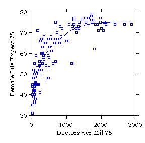
Nonlinearity in the regression function may appear in the scatter plot
of Y versus X, or in the residual plot. The residual plot often magnifies
nonlinearity (compared to the scatter plot) and makes it more noticeable.
A nonlinear trend may be revealed by using a nonparametric regression
technique such as LOWESS. The LOWESS algorithm estimates a curve
that represents the main trend in the data, without assuming a specific
mathematical relationship between Y and X. (This is why it is called
nonparametric.)
The next two exhibits show (1) a scatterplot of female life expectancy
against doctors per million for 137 countries in 1975, and (2) a plot of
the residuals of the regression of female life expectancy on doctors
per million. Note how the nonlinearity is magnified by the residual
plot, as compared to the plot of Y against X.
LOWESS (aka LOESS) was invented by William S. Cleveland (1994:168-180,
1993:94-101).
2. Linearity or Lack of Fit Test (Diagnostic, Formal, Limited Applicability)
There is a test of linearity of the regression function, called the lack
of fit test. This test requires repeat observations (called replications)
at one or more levels of X, so it cannot be performed with all data sets.
In essence it is a test of whether the means of Y for the groups of replicates
are significantly different from the fitted value ^Y on the regression
line, using a kind of F test. The test is explained in ALSM5e pp.
119-127; ALSM4e pp. 115-124.
3. Polynomial Regression (Remedy)
Some forms of non-linearity can be modeled by introducing higher powers
of X in the regression equation. Polynomial regression is a form
of multiple regression and is discussed in Module 6 - Polynomial Regression
& Interactions.
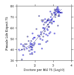
4. Transforming Variables To Linearize the Relationship (Remedy)
1. Error Variance Appears Constant
When the error variance appears to be constant, only X needs be
transformed to linearize the relationship. Some typical situations
are shown in the next exhibit.
The following exhibit shows an example of a non-linear regression function
that can be straightened by transforming X.
2. Error Variance Appears Not Constant
When the error variance does not appear constant it may be necessary
to transform Y or both X and Y. The next two exhibits show examples.
3. Transformation to Simultaneously Linearize the Relationship and
Normalize the Distribution of Errors
See Box-Cox transformation under 6.2 below.
3. Error Terms Do Not Have Constant Variance (Heteroskedasticity)
1. Funnel-Shape in in Residual Plot (Diagnostic, Informal)
Terminology:
homoskedasticity: s2
is
constant over the entire range of X (as specified by OLS assumptions)
heteroskedasticity: s2
is not constant over the entire range of X (departure from OLS assumptions)
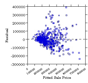
The regression model assumes homoskedasticity. Heteroskedasticity
may be manifested by a funnel or megaphone pattern like the following prototype
A real example is
Sometimes the funnel pattern is reversed, with greater error variance corresponding
to smaller values of X.
Q - Why is the variance in depression score lower for higher incomes and
vice-versa?
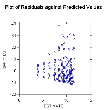
However, when the residual is plotted against ^Y the megaphone pattern
fans out to the right. (Why?)
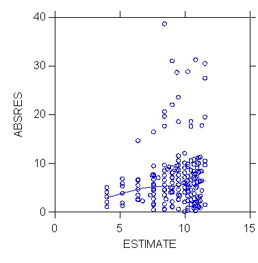
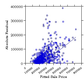
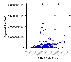
2. Plot of Absolute Residual |e| or Squared Residual e2
by ^Y (Diagnostic, Informal)
A pattern of heteroskedasticity can be detected informally by plotting
the absolute residual or the squared residual against ^Yi; adding
the linear fit or a LOWESS curve helps seeing the trend in the data:
3. Tests for Homoskedasticity (Constancy of s2
) (Diagnostic, Formal)
There are many tests of heteroskedasticity. Three formal tests of
constancy of the error variance will be discussed in Module 12 - Heteroskedasticity
& Weighted Least Squares:
-
the Brown-Forsythe Test (see ALSM5e pp. 116-118; not in ALSM4e)
-
the Breusch-Pagan aka Cook-Weisberg Test (see ALSM5e pp. 118-119;
ALSM4e p. 115)
-
the Goldfeld-Quandt test (Wilkinson, Blank, and Gruber 1996:274-277)
(The Breusch-Pagan aka Cook-Weisberg Test can be carried out in
STATA with the command hettest following the regress command.
An example will be shown in the hands-on session.)
4. Variable Transformation To Equalize the Variance of Y (Remedy)
See Section 6 below on Tukey's ladder of powers and the Box-Cox transformation.
Transformations of Y to make the distribution of residuals normal often
have the effect of also equalizing the variance of Y over the entire range
of X.
5. Weighted Least Squares (Remedy)
In rare cases where a variable transformation that takes care of unequal
error variance cannot be found, one can use weighted least squares.
In weighted least squares observations are weighted in inverse proportion
to the variance of the corresponding error term, so that observations with
high variance are downweighted relative to observations with low variance.
Weighted least squares is discussed in Module 12 - Heteroskedasticity &
Weighted Least Squares.
4. Error Terms Are Not Independent
1. Residual e by Time or Other Sequence (Diagnostic, Informal)
In time series data where observations correspond to successive time points,
errors can be autocorrelated or serially correlated.
Such a pattern can be seen in a plot of residuals against the time order
of the observations, as in the following prototype
The following real example shows residuals for a regression of the
divorce rate on female labor force participation (U.S. 1920-1996).
Note the characteristic "machine gun" tracking pattern. The residual
is plotted against the index of a case (corresponding to a year of observation).
Q - What year is the peak divorce residual?
Remedial techniques for lack of independence are discussed in Module
14 - Autocorrelation in Time Series Data.
2. Durbin-Watson Test of Independence (Diagnostic, Formal)
See Module 14 - Autocorrelation in Time Series Data.
5. Model Fits All But One Or A Few Outlier Observations
1. Outliers in Scatterplot or Residual Plot (Diagnostic, Informal)
Outliers may often (but not always) be spotted in a scatterplot or residual
plot.
Outlying observations may affect the estimate of the regression parameters,
as shown in the following exhibit.
Outlying observations may sometimes be identified in a box plot or stem-and-leaf
display of the residuals (see below).
2. Tests for Outlier and Influential Cases (Diagnostic, Formal)
An extensive discussion of outliers and influential cases is provided in
Module 10 - Outlying & Influential Observations.
6. Error Terms Are Not Normally Distributed
Non-normality of errors corresponds to a range of issues with different
degrees of severity. Kurtosis (fat tails) and skewness are more serious
than more minor departures from the normal. These features of the
distribution blend in with the problem of outlying observations.
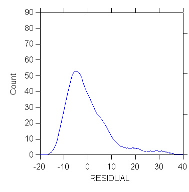
1. Box Plot, Stem-and-Leaf, and Other Displays of the Distribution
of e (Diagnostic, Informal)
Lack of normality (as well as some types of outlying observations) may
be diagnosed by looking at the distribution of the residuals using devices
such as a histogram, stem and leaf display, box plot, kernel density estimator,
etc. In the following examples see how the histogram of the
distribution appears normal but fat tails/outlying observations are revealed
in other displays.
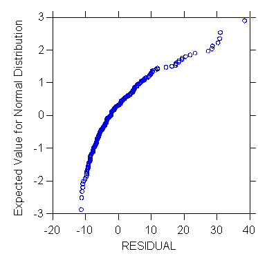
2. Normal Probability Plot of e (Diagnostic, Informal)
The normal probability plot is used to examine whether the residuals are
normally distributed. It is a plot of the residuals against their
expected values assuming normality. The expected values of the residuals
are obtained by first sorting them in increasing order of magnitude.
Then
EXPECTEDk = z((k - 0.5)/n) for k=1,...,n
where k is the rank of the residual such that k = 1 for the smallest value
of e and k = n for the largest, z((k - 0.5)/n) is the 100((k - 0.5)/n)
percentile of the standard normal distribution N(0,1).
When the residuals are normally distributed, the plot is approximately
a straight line.
Notes:
-
the textbook uses an alternative formula for EXPECTEDk that
yields similar results (ALSM5e pp. 110-112; ALSM4e pp. 106-108)
-
especially for relatively small samples, the normal probability plot may
not be conclusive concerning the normality of the distribution. A
formal correlation test (explained later) can be used. Alternatively,
Wilkinson, Blank, and Gruber (1996) suggest calibrating the normal probability
plot by generating probability plots for 10 random samples of size n from
a normal population, and judging visually whether the empirical plot "fits"
within this collection.
-
some computer implementation of the normal probability plot multiply z((k
- 0.5)/n) by the square root of MSE to obtain expected residuals with the
same scale as the original residuals (ALSM5e pp. 110-112; ALSM4e pp. 106-108).
The shape of normal probability plot reveals aspects of the distribution
of e.
The following exhibits show a full example of calculation of the probability
plot based on the Yule data set.
3. Correlation Test for Normality (Diagnostic, Formal)
The correlation test for normality is based on the normal probability plot.
It is the correlation between the residuals ei and their expected
values under normality. The higher the correlation, the straighter
the normal probability plot, and the more likely that the residuals are
normally distributed. The value of the correlation coefficient can
be tested, given the sample size and the a level
chosen, by comparing it with the critical value in Table B.6 in ALSM5e/4e.
A coefficient larger than the critical value supports the conclusion that
the error terms are normally distributed (ALSM5e pp. 115-116; ALSM4e p.
111).
Example: For the Yule data the correlation between residual and value
expected under the normality assumption is .981 with n=32. Table
B.6 in ALSM5e/4e gives the critical values for n = 30 of .964 with
a=.05.
Since r=.981 > .964 one concludes that the residuals are normally distributed.
4. Data Transformations Affecting the Distribution of a Variable
(Remedy)
This section relies extensively on Wilkinson, Blank, and Gruber (1996,
Chapter 22 pp. 695-713).
1. Standardizing a Variable - Does Not Affect Shape of Distribution
Common variable standardizations are the z-score and range standardization.
These transformations do not affect the shape of the distribution of the
variable (contrary to some popular beliefs).
The standardized value Z of Y is obtained by the formula
Z = (Y - Y.) / sY
where Y. and sY denote the sample mean and standard
deviation of Y, respectively.
The range-standardized value W of Y is obtained by the formula
W = (Y - YMIN) / (YMAX - YMIN)
where YMAX and YMIN denote the maximum and minimum
values of Y, respectively.
2. Transforming a Variable to Look Normally Distributed
Transformations of Y can be used to remedy non-normality of the error term.
a. Radical normalization with the rankit transformation
The rankit transformation transforms any distribution into a normal one.
It is the same as grading on the curve. It is the same as
finding the expected value of the residual in preparing a normal probability
plot.
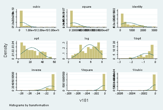
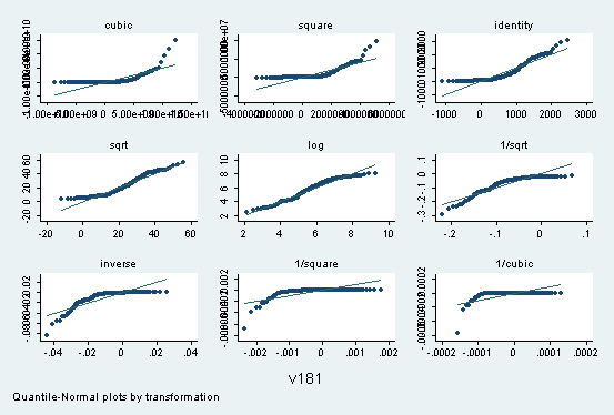
b. Tukey's ladder of powers
Tukey (1977) has proposed a ladder of powers spanning a range of
transformations to normalize the distribution of a variable in a data set.
c. Automatic choice of ladder of powers transformation with the Box-Cox
procedure
The family of power transformations in Tukey's ladder is of the form
Y' = Yl
where l is the power parameter. Some of
the principal steps of the ladder are
|
Lambda (l)
|
Transformation |
Name |
|
2
|
Y' = X2 |
square |
|
1
|
Y' = X |
identity |
|
.5
|
Y' = (X)1/2 |
square root |
|
0
|
Y' = log(X) |
logarithm (any base) |
|
-.5
|
Y' = 1/(X)1/2 |
inverse square root |
|
-1
|
Y' = 1/Y |
inverse |
but l can take any value in between.
In the simplest version the Box-Cox procedure estimates the parameter
l
by maximum likelihood so as to maximize the fit of the transformed data
Y' to a normal distribution. There is only one variable involved.
Example: Find the transformation of V181 (female life expectancy) that
best normalizes the distribution. STATA estimates lambda as
| lambda |
Std. Error |
z (same as t*) |
P{|Z|>z} |
CI Low |
CI Up |
Sigma |
| .1362285 |
.0660046 |
2.06 |
.039 |
.0068619 |
.265595 |
3.136496 |
The program does chi-square tests of 3 hypotheses on the value of lambda:
|
H0: l =
|
Chi-square |
P-value |
|
-1
|
300.88 |
.000 |
|
0
|
4.35 |
.037 |
|
1
|
140.35 |
.000 |
So estimated l (.1362285) is close to 0 (logarithm
transformation), but H0: l = 0 is
rejected at the .05 level (although not at the .01 level).
d. Box-Cox procedure to optimize the linear relationship between
X and Y
The Box-Cox procedure can also be used to transform Y and X in such a way
as to maximize their relationship. The procedure can estimate an
exponent
q (theta) of X as well as the exponent
l
(lambda) of Y. The complete model is thus
Yil = b0
+ b1Xiq
+ ei
The estimates l,
b0
, b1 and s2
can be found by maximizing the likelihood function shown in ALSM5e p. 135,
Equation 3.36; ALSM4e p. 135, Equation 3.35. There are now two variables
involved, Y and X. (The model generalizes to multiple regression,
with some limitations.)
In the following example v195 is Female Life Expectancy 1975 and v181
is Doctors per Million 181. The estimates are
| Coefficient |
Coefficient |
Std. Error |
z (same as t*) |
P{|Z|>z} |
95% CI Low |
95% CI Up |
| lambda |
.1772316 |
.0705726 |
2.51 |
0.012 |
.0389119 |
.3155514 |
| theta |
1.422054 |
.3605058 |
3.94 |
0.000 |
.7154761 |
2.128633 |
| V181 |
16.74134 |
Sigma = |
31.67667 |
|
|
|
Note that the exponent theta for X is 1.422, but the 95% CI includes
1.0 so one cannot reject the hypothesis that the optimal theta is 1.0 (optimal
transformation is no transformation).
On the Box-Cox procedure see ALSM5e pp. 134-137.
d. Arcsine transformation for proportions and percents
Proportions and percentages often produce a truncated and skewed distribution
when the mean is not near .5. The arcsine transformation corrects
these problems. Use
let ynew = 2*asn(sqr(P))
where P is a proportion. (Transform percentages to proportions by
dividing by 100 before applying transformation.)
e. Fisher's z transformation for correlation coefficients
Correlation coefficients often produce a truncated and skewed distribution
when the mean is not near 0. Fisher's z transformation (aka hyperbolic
tangent) normalizes such distributions. Use
let ynew = ath(R)
where R is a correlation between -1 and +1.
7. One or Several Important Predictor Variables Have Been Omitted
From Model
Plot of Residual e by Omitted Predictor Variable Z
Z is a potential predictor variable that is not included in the equation.
8. Simple Regression Diagnostics & Remedies in Practice
1. SYSTAT Examples
>USE
"Z:\mydocs\ys209\survey2b.syd"
[...deleted output...]
>regress
>model
total=constant+income
>save
resid/data
>estimate
Dep
Var: TOTAL N: 256 Multiple R: 0.210
Squared multiple R: 0.044
Adjusted
squared multiple R: 0.040 Standard error of estimate: 8.728
Effect
Coefficient Std Error Std Coef
Tolerance t P(2 Tail)
CONSTANT
11.811 0.948
0.000 . 12.461
0.000
INCOME
-0.120 0.035
-0.210 1.000 -3.425
0.001
Analysis
of Variance
Source
Sum-of-Squares df Mean-Square
F-ratio P
Regression
893.479 1 893.479
11.729 0.001
Residual
19348.271 254 76.174
***
WARNING ***
Case
256 is an outlier (Studentized
Residual = 4.598)
Durbin-Watson
D Statistic 0.659
First
Order Autocorrelation 0.631
Residuals
and data have been saved.
>use
resid
SYSTAT
Rectangular file Z:\mydocs\s208\resid.SYD,
created
Mon Jan 20, 2003 at 10:04:34, contains variables:
ESTIMATE
RESIDUAL LEVERAGE COOK
STUDENT SEPRED
ID
SEX AGE
MARITAL EDUCATN
EMPLOY
[...deletd
output...]
>let
absres = abs(residual)
>plot
absres*estimate/stick=out smooth=lowess
>den
residual/stick=out kernel
>pplot
residual/stick=out
>rem
calculate expected residuals under normality explicitly
>rem
to do correlation test
>sort
residual
256 cases and 56 variables processed.
>let
resrank = case
>list
residual resrank/n=10
Case number RESIDUAL
RESRANK
1 -11.212
1.000
2 -11.092
2.000
3 -10.973
3.000
4 -10.733
4.000
5 -10.733
5.000
6 -10.494
6.000
7 -10.015
7.000
8 -9.733
8.000
9 -9.571
9.000
10 -9.536
10.000
>let
expres = zif((resrank - 0.5)/256)
>rem
next plot should be same as pplot command
>plot
expres*residual/stick=out
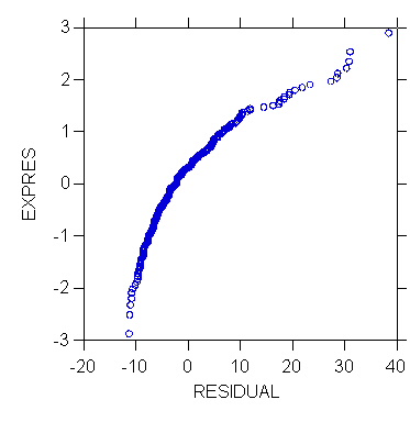
>corr
>pearson
expres*residual
Pearson
correlation matrix
RESIDUAL
EXPRES
0.926
Number
of observations: 256
>rem
test for normality using correlation test and
>rem
ALSM5e Table B.6
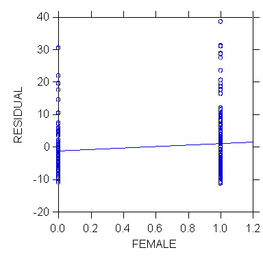
>plot
residual*female/stick=out smooth=linear
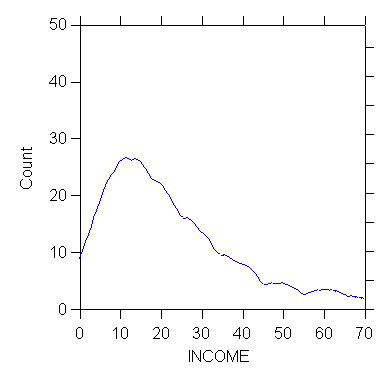
>den
income/stick=out kernel
>den
income/stick=out kernel
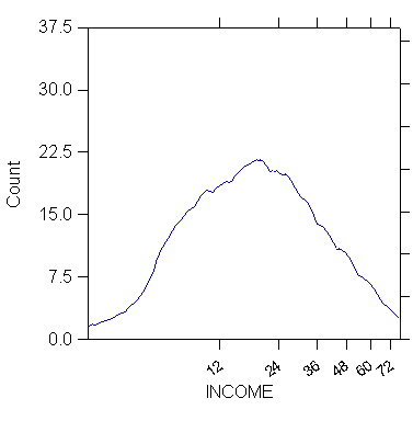
>rem
the kernel density of income is "normalized" by setting the power
>rem
exponent interactively after double-clicking on the graph, as shown
>rem
in following picture
>rem
this yields the kernel density with power exponent = 0.2
>USE
"Z:\mydocs\ys209\world209.syd"
[...deleted output...]
>plot
v195*v181/stick=out smooth=lowess
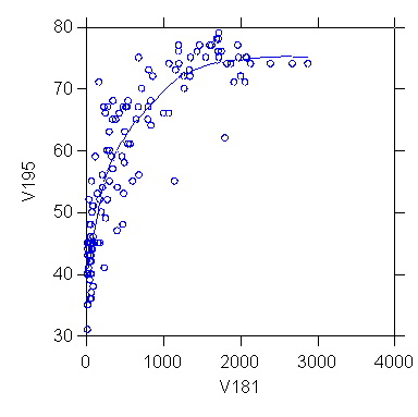
>rem scatterplot
with LOWESS curve shows strong non-linear
>rem pattern; relationship
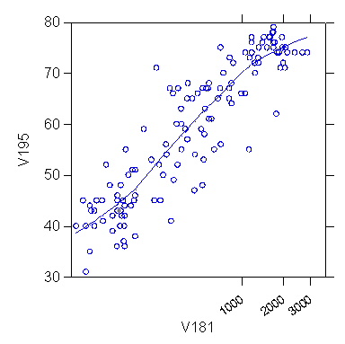
"straightend" by setting power
>rem exponent of
V181 to 0.2 interactively after double-
>rem clicking on
graph
>plot
v195*v181/stick=out smooth=lowess
2. STATA Examples
(By Catherine Harnois and
Cheol-Sung Lee, TAs in Spring 2003.)
We
highly recommend the UCLA STATA module for diagnostics
. use "C:\Stata\auto.dta",
clear
*1978 Automobile Data
. boxcox mpg, nolog
level(95)
Transform: (mpg^L-1)/L
L [95% Conf. Interval]
Log Likelihood
----------------------------------------------------
-0.3584 -1.1296 0.4078
-123.2664
Test: L == -1 chi2(1) =
2.68 Pr>chi2 = 0.1018
L == 0 chi2(1) =
0.82 Pr>chi2 = 0.3649
L == 1 chi2(1) =
12.25 Pr>chi2 = 0.0005
*nolog level(95) tells
Stata not to display the iterations log but to include
a 95% confidnence
interval. The interval rejects the hypothesis that the best
transformation
is no transformation.
*next create a new variable
newmpg based on the optimal exponent found by boxcox procedure
. gen newmpg = (mpg^(-0.3584)
- 1)/(-0.3584)
*next compare distributions
of mpg and newmpg
. graph mpg, bin(10)
ylabel xlabel norm t1(raw data)
.
graph newmpg, bin(10) ylabel xlabel norm t1(transformed data)
.
kdensity mpg, normal border
.
kdensity newmpg, normal border
.
ksm mpg weight, lowess xlab ylab border
.
ksm newmpg weight, lowess xlab ylab border
. stem mpg
Stem-and-leaf plot for
mpg (Mileage (mpg))
1t | 22
1f | 44444455
1s | 66667777
1. | 88888888899999999
2* | 00011111
2t | 22222333
2f | 444455555
2s | 666
2. | 8889
3* | 001
3t |
3f | 455
3s |
3. |
4* | 1
. ladder mpg
Transformation
formula
Chi-sq(2) P(Chi-sq)
------------------------------------------------------------------
cube
mpg^3
43.59 0.000
square
mpg^2
27.03 0.000
raw
mpg
10.95 0.004
square-root
sqrt(mpg)
4.94 0.084
log
log(mpg)
0.87 0.647
reciprocal root
1/sqrt(mpg)
0.20 0.905
reciprocal
1/mpg
2.36 0.307
reciprocal square
1/(mpg^2)
11.99 0.002
reciprocal cube
1/(mpg^3)
24.30 0.000
In this formula, m=mu
and s=the standard deviation and I is the observation number.
.
pnorm mpg
.
pnorm newmpg
. regress mpg weight
Source |
SS df
MS
Number of obs = 74
---------+------------------------------
F( 1, 72) = 134.62
Model |
1591.9902 1 1591.9902
Prob > F = 0.0000
Residual | 851.469256
72 11.8259619
R-squared = 0.6515
---------+------------------------------
Adj R-squared = 0.6467
Total |
2443.45946 73 33.4720474
Root MSE = 3.4389
------------------------------------------------------------------------------
mpg | Coef. Std. Err.
t P>|t| [95%
Conf. Interval]
---------+--------------------------------------------------------------------
weight |
-.0060087 .0005179 -11.603 0.000
-.0070411 -.0049763
_cons |
39.44028 1.614003 24.436
0.000 36.22283 42.65774
------------------------------------------------------------------------------
.
fpredict yhat
.
fpredict e,resid
.
graph e yhat
.
rvfplot, oneway twoway box yline(0) ylabel xlabel
. hettest
Cook-Weisberg test for
heteroscedasticity using fitted values of mpg
Ho: Constant variance
chi2(1) = 11.05
Prob > chi2 = 0.0009
. ovtest
Ramsey RESET test using
powers of the fitted values of mpg
Ho: model has no omitted variables
F(3, 69) = 1.77
Prob > F = 0.1616
Appendix - Mathematical Functions
Mathematical and Satistical Functions Available in SYSTAT
Mathematical and Satistical Functions Available in STATA
Please consult STATA Manual
Last modified 30 Jan 2006
![Exhibit: Female life expectancy by literacy: residual by estimate [m3002.gif]](m3002.gif)
![Exhibit: Plot of female life expectancy against doctors per million ca. 1975, with LOWESS curve (repeat) [m16004.jpg]](m16004.jpg)
![Exhibit: Residual plot for the regression of female life expectancy against doctors per million ca. 1975, with LOWESS curve [m16005.jpg]](m16005.jpg)
![Exhibit: Prototype nonlinear plots with equal error variance (ALSM5e F3.13 p. 130; ALSM4e F3.13 p. 127) [m3009.gif]](m3009.gif)
![Exhibit: Prototype nonlinear plots with unequal error variance (ALSM5e F3.15 p. 132; ALSM4e F3.15 p. 130) [m3010.gif]](m3010.gif)
![Exhibit: Transformations on scatterplots to linearize a relationship (WBG F22.4 p. 705) [m3014.gif]](m3014.gif)
![Exhibit: Plot of TOTAL (depression scale) by INCOME showing greater variance in depression score for smaller income values [m3039.jpg]](m3039.jpg)
![Exhibit: Residual plot for regression of TOTAL (depression scale) on INCOME [m3037.jpg]](m3037.jpg)
![Exhibit: Plot of absolute residuals against estimate for regression of TOTAL (depression scale) on INCOME [m3038.jpg]](m3038.jpg)
![Exhibit: Residuals of divorce rate on female labor force participation, by file index (year) -- U.S. 1920-96 [m3054.jpg]](m3054.jpg)
![Exhibit: Distorting effect of outlier (ALSM5e F3.7 p. 109; ALSM4e F3.7 p. 104) [m3020.gif]](m3020.gif)
![Exhibit: Effect of outlying observation on estimated regression line (NWW Figure 19.9 p. 590) [m16008.gif]](m16008.gif)
![Exhibit: Distribution of residuals of regression of female life expectancy on literacy rate (v227) [m16007.jpg]](m16007.jpg)
![Exhibit: Stem and leaf plot of residuals [m3021.gif]](m3021.gif)
![Exhibit: DOT ("DIT") plot and box plot [m3022.gif]](m3022.gif)
![Exhibit: Normal probability plot of residuals of female life expectancy on literacy rate [m3023.gif]](m3023.gif)
![Exhibit: Normal probability plots (ALSM5e F3.9 p. 112; ALSM4e F3.9 p. 108) [m3024.gif]](m3024.gif)
![Exhibit: Plot of PAUP by OUTRATIO [m3033.gif]](m3033.gif)
![Exhibit: Normal probability plot of residuals for the regression of PAUP on OUTRATIO [m3055.jpg]](m3055.jpg)
![Exhibit: Standardizing a variable (WBG F22.1 p. 697) [m3011.gif]](m3011.gif)
![Exhibit: Normalizing a variable (WBG F22.2 p. 699) [m3012.gif]](m3012.gif)
![Exhibit: Ladder of power transformations to normalize a variable (WBG F22.3 p. 703) [m3013.gif]](m3013.gif)
![Exhibit: Female life expectancy by literacy: residual by other variable [m3025.gif]](m3025.gif)
![Exhibit: SYSTAT arithmetic functions (SYSTAT 6.0 Data p. 119) [m3026.gif]](m3026.gif)
![Exhibit: SYSTAT distribution functions (SYSTAT 6.0 Data p. 143) [m3027.gif]](m3027.gif)