Soci 709 (formerly 209) Module 7 - QUALITATIVE
INDEPENDENT VARIABLES
1. INDICATOR VARIABLES
An indicator (or binary variable)
is a variable that can have only two values, 0 or 1.
Indicator variables are used to represent
qualitative
(or nominal or categorical) variables.
A qualitative (nominal or categorical) variable
with k classes is represented in the regression model by k-1
indicators.
(Indicators are also called "dummy variables"
but this usage is unfortunate as it incorrectly implies that indicators
are "fake" variables in some sense, which they are not.)
Regression models with indicator variables
are very important in part because they represent a bridge between regression
analysis and a set of statistical techniques called analysis of variance
(ANOVA) and analysis of covariance (ANCOVA) - see the second part
of ALSM5e or ALSM4e. All ANOVA or ANCOVA models can be represented
as regression models with suitably defined indicators.
Examples:
Note on naming an indicator variable: consider
naming an indicator variable after the category that has the value 1.
For example a variable that 1 for female, and 0 for male can be named FEMALE;
the meaning remains clear. If the variable is named SEX or GENDER, you
will forget which one is 1 and which one is 0 six months later.
Detailed example 1: Restaurants Study
In a study of restaurants, volume of sales (in
dollars) is the dependent variable. One independent variable (x1)
is Number of Households in the area (a regular continuous variable). The
other independent variable is restaurant location, a qualitative variable
with 3 categories: Highway, Shopping Mall, or Street. The indicators
used are
X2 = 1 if Shopping Mall
location, 0 otherwise
X3 = 1 if Street location, 0 otherwise
Highway location does not have an indicator associated
with it. Highway location is called the reference, baseline,
or omitted category or class. The reference class is the class
for which every indicator is set to zero. The restaurant data are
set up as in the next exhibit.
The regression model is
yi = b0
+ b1Xi1
+ b2Xi2
+ b3Xi3
+ ei
where Xi1 is and Xi2
and Xi3 are the two location indicators.
The meaning of the coefficients is revealed
by examining the regression function
E{Y} = b0
+ b1X1
+ b2X2
+ b3X3
There are three cases, depending on location
Values of Regression Function E{Y}
= b0
+ b1X1
+ b2X2
+ b3X3
for Different Restaurant Locations
|
Restaurant Location
|
Values of Indicators
|
Regression Function
|
|
Highway
|
E{Y} = b0
+ b1X1
+ b2(0)+
b3(0) |
E{Y} = b0
+ b1X1 |
|
Shopping Mall
|
E{Y} = b0
+ b1X1
+ b2(1)
+ b3(0) |
E{Y} = ( b0
+ b2)
+ b1X1 |
|
Street
|
E{Y} = b0
+ b1X1
+ b2(0)
+ b3(1) |
E{Y} = (b0
+ b3)
+ b1X1 |
The table shows that b2
and b3
represent the differences in intercept for Shopping Mall and Street
location, respectively, relative to Highway (the omitted category).
This can be seen by plotting the regression function for the three locations.
Detailed example 2: Depression Scores Study
Models of the depression score with the Afifi
& Clark (1984) data set.
Number of Categories
A categorical variable with k classes (categories)
is represented by k-1 indicators, with one category omitted.
Using k indicators to represent a categorical variable with k classes
would make the X'X matrix singular, so b
cannot be estimated.
2. INDICATOR MODELS WITH INTERACTIONS
The indicator model with interaction is discussed in the context of a
substantive example.
Detailed example
(From Hamilton 2006: pp. 180--185.)
Units are states of the
U.S. Variables are
y (dependent variable) is csat (=mean composite SAT score by
State)
x1 is percent = percent HS graduates taking SAT (a
continuous variable)
x2 is reg2 = 1 for North East Region, 0 for other regions
(an indicator variable)
The coefficient of a continuous independent variable
y may be allowed to vary as a function of an indicator
variable by using an interaction term. The response function for the interaction model becomes
E{y} = b0
+ b1x1
+ b2x2
+ b3x1x2
where y = mean composite state SAT score, x1
= percent HS graduates taking the SAT and x2 = North-East indicator (1 if
state is in North-East, 0 otherwise).
Again to understand the meaning of the coefficients
one must examine the regression (response) function for each category of
the qualitative variable:
Values of Regression Function E{y}
= b0
+ b1x1
+ b2x2
+ b3x1x2
for Different States
|
Region
|
Values of x2 and x1x2
|
Regression function
|
| not North-East (x2=0) |
E{y} = b0
+ b1x1
+ b2(0)
+ b3(0) |
E{y} = b0
+ b1x1 |
| North-East (x2=1) |
E{y} = b0
+ b1x1
+ b2(1)
+ b3x1(1) |
E{y} = (b0
+ b2)
+ (b1+
b3
)x1 |
STATA (V9) commands are:
use "Z:\mydocs\s209\hamiltonv9\states.dta", clear
describe region
tabulate region
tabulate region, gen(reg)
* gen(reg) creates 4 (0,1) indicators, for each region
regress csat percent reg2
gen nexpct=reg2*percent
*nexpct is reg2 by percent interaction term
regress csat percent reg2 nexpct
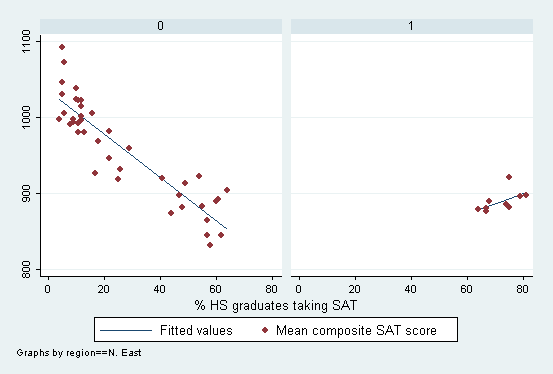
*next graph is equivalent to conditional effects plot
graph twoway lfit csat percent || scatter csat percent || , by(reg2)
The estimated model is (t-ratios in parentheses):
| y = |
1035.519 |
-2.859x1 |
-241.357x2 |
4.180(x1x2) |
R2=.843 |
n=50 |
| |
(150.01) |
(-14.06) |
(-2.07) |
(2.58) |
|
|
The
significant interaction effect suggests that percent (x1) affects csat negatively
in most regions but positively in the North East. (Is the effect
of North East of the reinforcement or interference type?).
Thus in the interaction model both the intercept and
the slope of the continuous variable x1 differ across types of firm.
This can be visualized with a conditional effects that compares
the regression functions for the two types of states.
3. COMPARISON OF TWO OR MORE REGRESSION
FUNCTIONS
A very common research strategy is to study the
similarities and differences between regression models for 2 or more populations.
Example: a social scientist wants to
compare a regression model of earnings as a function of education and experience
(time in the labor force) for full-time year-round employed men and women,
perhaps to detect any discriminatory treatment suffered by one of the groups
Example: a sociologist wants to compare
the status attainment process in the 1960s and 1990s by estimating the
same model of occupational prestige as a function of education and family
background characteristics (F's Education, M's Education, F's Occupation,
etc.) using subjects in the same age range in the 1960s and 1990s, perhaps
to monitor any trend of increasing or decreasing social mobility between
the two periods
Example: a much more exciting project is a
comparison of two production lines for making soap bars. For each
production line, the relation of interest is that between the amount of
scrap for the day (the dependent variable) and the speed of the production
line. A symbolic scatter plot of Amount of Scrap against Line Speed
suggests that the regression relation is not the same for the two production
lines (next exhibit).
When it is reasonable to assume that the error
term variances in the regression models for the different populations are
equal, one can use indicator variables to test the equality of the different
regression functions. (When the variances are not equal, a suitable
transformation of Y can equalize them approximately. See NKNW p.
472 for an example of formal test of the equality of the error variances
for two populations.) This is done by considering the different populations
as classes of a predictor variable, define indicator variables for the
different populations, and estimating a single regression model containing
appropriate interaction terms, similar to the insurance innovation interaction
model above.
For the Soap Production data define an interaction
model with regression function
E{Y} = b0
+ b1X1
+ b2X2
+ b3X1X2
where Y = Amount of Scrap, X1 = Line
Speed, and X2 is Line 1 (=1 if production line 1, 0 if production
line 2).
The estimated regression model is (t-ratios
in parentheses)
^Y = 7.57 + 1.322X1 + 90.39X2
- .1767X1X2
(.36) (14.27)
(3.19) (-1.37)
so one concludes that the slope of the relationship
between Amount of Scrap and Speed does not differ across production lines
(b3 is non significant with t* = -1.37) but that the intercepts
are significantly different, so that Amount of Scrap is overall higher
in Line 1 than in Line 2 (b2 is significant with t* = 3.19).
(One can formally test the equality of the
regression lines with the joint test of H0: b2
= b3
= 0 ; see NKNW pp. 472-473. We will study joint testing later.)
Example: comparing the return to education
(in terms of income) for men and women, using the survey2.syd data set.
Q -- What kind of substantive research often uses
models like the ones in the last exhibit?
4. PIECEWISE LINEAR REGRESSION & DISCONTINUITIES
1. Piecewise Regression -- Change of Slope
Point Known
Indicator variables can be used to model situations
in which the slope of the regression of Y on X differs for two ranges
of X, as in the following exhibit:
Assuming that Xp (the point where
the slopes change) is known, the piecewise
linear relation is represented by a regression model with response function
E{Y} = b0
+ b1X1
+ b2(X1
- 500)X2
where Y = Unit Cost, X1 = Lot Size,
X2 = 1 if X1>500, = 0 otherwise, and Xp
= 500.
One can convince oneself that this function
represents the piecewise linear relation by examining the response function
separately for the range X1 <= 500 and the range X1
> 500, as shown in the next exhibit
The model can be estimated from the data
The estimated regression function is
^Y = 5.89545 - .00395X1
- .00389(X1 - 500)X2
Piecewise linear modelling can be easily extended
to more than 2 pieces. See NKNW p. 477.
When Xp is not known, one may
-
attempt to guess its position from the scatterplot
-
use non-linear regression techniques to estimate
Xp together with the other parameters of the model iteratively.
The following link shows a complete piecewise
linear analysis using the Lerner data.
2. Piecewise Regression -- Change of Slope
Point Unknown
When the xp is not known, xp
and the regression function can be estimated simultaneously using nonlinear
least-squares.
The following exhibit shows how to estimate a
piecewise regression model when xp is not known, using STATA and the
Lerner data. Note that the estimate of xp is 49, which is
a bit less than the value suggested by the lowess regression curve (about 60),
although the 95% CI for xp is wide so 60 is not an implausible
estimate of the "elbow" of the relationship (28.9053 to 69.09471).
3. Discontinuity in Regression Function
One can also use indicators to model discontinuous
piecewise linear regression relations, as in the following exhibit.
See NKNW pp. 477-478 for details.
5. INDICATORS VERSUS QUANTITATIVE VARIABLES
1. Indicators Versus Allocated Codes
Qualitative variables with ordinal categories
can often be represented either by allocated codes or by indicators.
For example, persons of Hispanic origin might be asked the question "How
often do you use Spanish at home?" with response categories Frequently,
Occasionally, Never. The variable may be coded with allocated codes
in variable X1, or with two indicators X2 and X3:
Alternative codings of frequency of Spanish use at home:
X1: allocated codes; X2 and X3:
indicators
| Class |
X1
|
X2: Frequent User
|
X3: Occasional User
|
| Never |
1
|
0
|
0
|
| Occasionally |
2
|
0
|
1
|
| Frequently |
3
|
1
|
0
|
Using allocated codes X1 in the model
with response function E{Y} = b0
+ b1X1
constrains differences in response function among classes to be the same,
as can be seen by writing the response functions for each category of use:
Never: E{Y} = b0
+ 1. b1
Occasionally: E{Y} = b0
+ 2. b1
Frequently: E{Y} = b0
+ 3. b1
Therefore
E{Y|Frequently} - E{Y|Occasionally}
= E{Y|Occasionally} - E{Y|Never} = b1
(Say this in words.) The assumption of constant
differences in effect among contiguous classes may or may not be substantively
plausible.
Using indicators X2 and X3
in the model with response function E{Y} = b0
+ b2X2
+ b3X3
allows differences in response functions among classes to be different:
E{Y|Frequently} - E{Y|Never} = b2
E{Y|Occasional} - E{Y|Never} = b3
E{Y|Frequently} - E{Y|Occasional} = (b2
-
b3)
Thus in the indicators model the effects of the
classes are not arbitrarily restricted. On the other hand categories
use up more degrees of freedom (k-1 variables) than allocated codes
(one variable).
2. Indicators Versus Quantitative Variable
For the same reasons, it may be useful to use
a set of indicators rather than continuous values even when a variable
is inherently quantitative.
Example: to study the relationship of earnings
with age, age in years is represented by a set of indicators corresponding
to 5-years categories 20-24, 25-29, 30-34, etc. Using indicators
may allow for a better "tracking" of the non-linear relationship between
Y (earnings) and X (age). The disadvantage of indicators is that
more degrees of freedom are consumed (k-1 indicators versus 1
continuous variable), but this is not a problem with large data sets.
Example: The variable EDUCATN in the Afifi
& Clark (1984) data set can be viewed as an allocated code or as a
quantitative variable. One can create a set of indicators from the
code corresponding to various levels of education. The next exhibit
compares models of the effect of education on income using years of education
(as a quantitative variable), on one hand, and using a set of indicators,
on the other.
3. Alternative Coding for Indicators
Alternatives to the coding of a qualitative variable
with k-1 (0,1) indicators and a constant term are
-
k-1 indicators coded (0,1,-1) and a constant
term. This is the same as (0,1) coding except that observations corresponding
to the reference class are coded -1 for all the indicators. One can
show that the intercept then represents an average intercept for
the classes. This type of coding is common in ANOVA.
-
k (0,1) indicators with no constant term.
The coefficients of the indicators are then interpreted as class-specific
intercepts.
See ALSM5e ???; ALSM4e pp. 481-482 and Section
16.11 (pp. 696-701) for discussion of the relationship between regression
and ANOVA.
6. QUASI-INDICATORS: DF ANALYSIS OF FAMILY DATA
This section is to be added later.
Last modified 27 Feb 2006