Soci709 (formerly 209) Module 14 - AUTOCORRELATION IN TIME SERIES DATA
Resources:
ALSM5e pp 481--498; ALSM4e pp 497--516
Hamilton 2006 pp. 339-360 (especially commands tsset date and prais y
x1 x2)
1. AUTOCORRELATION OF ERRORS: NATURE OF
THE PROBLEM
Time series data are observed on the same unit
(individual, country, firm, etc.) at n points in time. EX:
-
yearly divorce rate in the U.S. from 1922 to present
-
quarterly profits of a company
-
income inequality in the U.S. measured each year
from 1964 to present
-
daily atmospheric pollen count in Chapel Hill
since first recorded, etc.
In regression models using time series data the
errors are often correlated over time (they are said to be autocorrelated
or serially correlated).
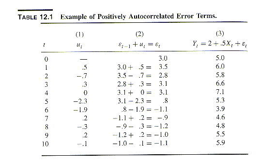
NKNW illustrate the problems caused by correlated
errors with simulated data generated with the model:
-
Yt = b0
+ b1Xt
+ et
-
et = et-1
+ ut
-
Xt represents "time", so that X1=1,
X2=2, etc.
-
b0 = 2;
b1
= .5
-
e0 (et
prior to beginning the process) = 3
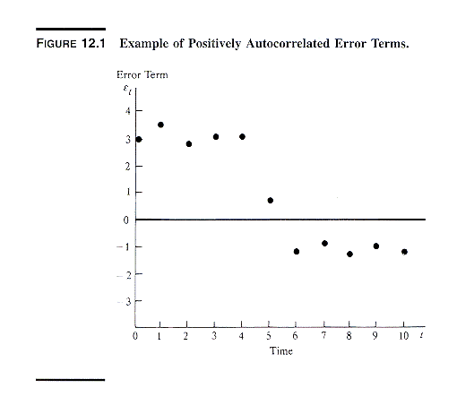
The simulated data are shown in the next exhibit.
As seen in the next exhibit, the errors et
are positively correlated.
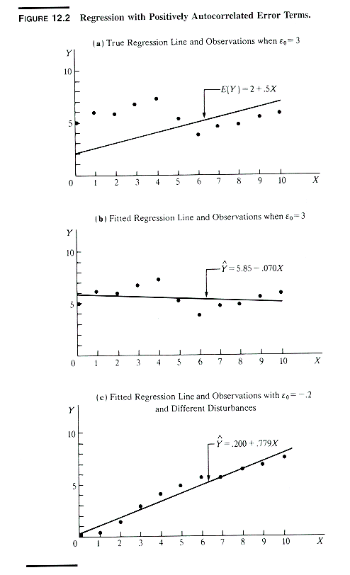
Because of serial correlation
-
the OLS and true regression lines may differ sharply
from sample to sample depending on the initial disturbance e0
(compare (a), (b) and (c) in next exhibit)
-
MSE may underestimate true variance of et
(compare variability of residuals around regression line in (a) and (b)
in next exhibit); thus standard errors of estimate of the regression coefficients
may also be underestimated
These patterns can be seen in the next exhibit
In general, serial correlation of the disturbances
may have the following effects with OLS estimation
-
estimated regression coefficients are still
unbiased but no longer minimum variance (= inefficient)
-
MSE (the OLS estimate of s2)
may underestimate the true variance of errors
-
s{bk} may underestimate true standard
error of estimate
-
thus, statistical inference using t and F is no
longer justified
2. AUTOCORRELATION DIAGNOSTICS
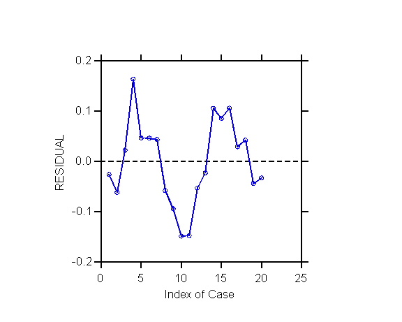
1. Plot of Residuals Against Time or Sequential
Order
An informal diagnostic of autocorrelation of errors
is to plot the residuals from the OLS regression against time or against
the sequential order of the observation in the file (after checking that
observations are in fact arranged in chronological order!). Connecting
the points with a dotted line makes any pattern of autocorrelation more
conspicuous. Look for evidence of "tracking", in which residuals
corresponding to adjacent time points have similar values. (Some
people say to look for a pattern like that made by bullets fired from a
machine gun.)
Exhibit: Index plot
(= time plot) of residuals for Blaisdell data
2. The Wald-Wolfowitz Runs Test
The Wald-Wolfowitz runs test is a non-parametric
test that detects serial patterns in a run of numbers. Applied to
the residuals of the OLS regression, a significant test indicates the presence
of sequences of positive or negative residuals longer than expected by
chance alone. Such long sequences of residuals above or below zero
is what one would expect if the errors are "tracking" because of autocorrelation.
For the Blaisdell data the test is significant
(p=.006) so one concludes that the errors are correlated.
3. The Durbin-Watson Test
The Durbin-Watson (D-W) test is the most commonly
used test of autocorrelation of residuals.
The D-W D statistic is calculated from the
ordinary OLS residuals et = Yt - ^Yt as
D = St=2
to n (et - et-1)2 / St=1
to n et2
where n is the number of cases.
To understand the D-W formula consider that
-
when et and et-1 are correlated
they have similar values
-
thus when et and et-1 are
correlated the terms (et - et-1)2 are
small and the numerator of D is small (while the denominator is the same
no matter how much autocorrelation there is)
-
thus small values of D (close to zero) indicate
serial correlation
The D-W test setup is
H0: r
= 0
H1: r
> 0
Table B7 gives critical values dL and
dU such that
if D > dU conclude H0
(r = 0)
if dL <= D <= dU
the test is inconclusive
if D < dL conclude H1
(r > 0)
Example: SYSTAT routinely reports the D-W
D statistic with every regression (D has no meaning unless observations
are sequentially ordered). For the Blaisdell data D = .735.
Table B7 for n=20 and p-1=1 gives dL=.95 and dU=1.15.
Since .735 < .95 = dL one concludes H1 (errors
are autocorrelated).
3. REMEDIAL MEASURES FOR AUTOCORRELATION
1. Add Omitted Predictors to Model
Autocorrelation is caused by unmeasured variables
that have similar values from period to period. Identifying these
variables and including them in the model may eliminate the serial correlation.
Some of these substantive omitted variables may be "simulated" by adding
to the model
-
a linear or exponential trend
-
seasonal indicators
If adding a trend or seasonal indicators gets
rid of the autocorrelation, this is by far the best solution to the problem.
2. The First-Order Autoregressive Error
Model With Generalized Least Squares Estimation
1. First-Order Autoregressive Error Model
The model is
Yt = b0
+ b1Xt1
+ b2Xt2
+ ... + bp-1Xt,p-1
+ et
et =
ret-1
+ ut
where
|r|
< 1 (r
is Greek "rho" and denotes the autocorrelation parameter)
ut is i.i.d. ~ N(0, s2)
One can show the following consequences of model
assumptions (see ALSM4e pp. 501-502; try to express these relationships in
words):
-
E{et}
= 0
-
s2{et}
= s2/(1-r2)
-
s{et,
et-1}
= r(s2/(1-r2))
-
r{et,
et-1}
= s{et,
et-1}/(s{et}s{et-1})
= r
-
r{et,
et-s}
= rs
Thus the variance-covariance matrix of e
is non-diagonal with a specific structure; s2{e}
=
| k |
kr |
kr2 |
... |
krn-1 |
| kr |
k |
kr |
... |
krn-2 |
| ... |
... |
... |
... |
... |
| krn-1 |
krn-2 |
krn-3 |
... |
k |
where
k = s2/(1-r2)
( k is Greek
"kappa")
(This is why the model is called "generalized",
as in "generalized least squares"; see Module 12.)
Even though the first-order autoregressive
model is simple, it is often a good approximation of actual situations.
2. Generalized Least Squares Estimation
Using Transformed Variables
Assume (for the sake of argument) that one knows
the value of r.
Define the transformed variables
Yt' = Yt - rYt-1
Xtk' = Xtk - rXt-1,k
Then one can show that the regression
Yt' = b0'
+ ... + bk'Xtk'
+ ... + ut
based on the transformed variables has error term
ut which is no longer serially correlated, and that bk
= bk'
except that b0'
= b0(1-r)
(see NKNW pp. 508-509). Thus if one knows r
one can get rid of the serial correlation by using OLS with the transformed
data.
(This transformation can be derived from the
application of GLS estimation to the non-diagonal variance-covariance matrix
of e generated
by the autocorrelation. So the transformation is a special case of
GLS estimation.)
In practice the value of r
is unknown. The 3 classical methods of estimation in the presence
of autocorrelation discussed next (Cochrane-Orcutt, Hildreth-Lu, first
differences) are all based on transforming the variables, using alternative
ways of estimating r.
3. Cochrane-Orcutt Procedure
The Cochrane-orcutt procedure is
-
do an OLS regression of Yt on the Xtk
and calculate the residuals et
-
estimate the autocorrelation r
as
r = St=2
to n et-1et / St=2
to n et-12
-
use r to transform the variables into Yt'
and Xtk' using formula above; do an OLS regression of Yt'
on the Xtk'
-
if the D-W test still indicates serial correlation,
reestimate r using residuals computed using the original variables Yt
and Xtk and the regression coefficients estimated from the (last)
transformed regression; go to 3.
The following exhibits show the Cochrane-Orcutt
procedure with the Blaisdell data.
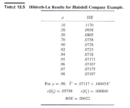
4. Hildreth-Lu Procedure
The Hildreth-Lu procedure searches for the estimate
of r that minimizes
the sum of squared errors of the transformed regression, i.e.
SSE = S(Yt'
- ^Yt')2
(Hilderth-Lu is similar to the Box-Cox procedure
to estimate the parameter l
of a power transformation of Y.)
One can search for the optimal r
by calculating the transformed regression for closely spaced values of
r
and choosing the one with smallest SSE, as shown in NKNW.
One can also estimate r
and the regression coefficients simultaneously using iterative methods
(nonlinear least squares). This can be done using the NONLIN module
of SYSTAT, as shown in the exhibit analyzing the Blaisdell data.
Exhibit: (REPEAT) Replication
of Cochrane-Orcutt, Hildreth-Lu, & first differences procedures for
Blaisdell data
5. First Differences Procedure
First differences is the simplest transformation
procedure as it implicitly assumes r
= 1. This assumption is often approximately justified because
-
estimates of r
are often close to 1
-
the relationship of SSE with r
is often "flat" (as seen in the Hildreth-Lu procedure: see ALSM4e Table 12.5
p. 513) for values of r
near the optimum, so the estimate of r
does not need to be exact
The first differences transformation is thus
Yt' = Yt - Yt-1
Xtk' = Xtk - Xt-1,k
The first differences procedure involves two
regressions with the transformed data:
-
a first regression without a constant term
to estimate the regression coefficients (since the first differences transformation
"wipes out" the constant term)
-
a second regression with a constant term
to recalculate the D-W D statistic only (because the D-W formula requires
a constant in the model)
6. Comparison of the 3 Transformation Methods
Results of the 3 transformation methods (compared
with OLS) are shown in the following table.
Regression results for 4 estimation methods
(SYSTAT) - Blaisdell data (compare with ALSM5e <>, ALSM4e Table 12.7 p. 516 - some figures differ slightly)
|
b1 |
s{b1} |
t-ratio |
r |
MSE |
| Cochrane-Orcutt |
.1738 |
.0029 |
59.42 |
.626 |
.004515 |
| Hildreth-Lu (nonlinear LS) |
.1605 |
.0079 |
20.24 |
.959 |
.004479 |
| First differences |
.1685 |
.0051 |
33.06 |
1.0 |
.004815 |
| OLS |
.1763 |
.0014 |
122.0 |
0.0 |
.007406 |
7. STATA Commands
4. COMPREHENSIVE EXAMPLE: U.S. DIVORCE RATE
1920-1970, 1920-1997
1. SYSTAT Analysis
The following exhibit present examples of the
Cochrane-Orcutt, Hildreth-Lu (using nonlinear least squares), and first
differences methods applied to an analysis of the divorce rate in the U.S.
from 1920 to 1970.
As a substantive epilogue the next 3 exhibits relate to a model of the
divorce rate that is more elaborate than one previously shown, as it includes
a measure of the birth rate (women 15-44) and military personnel per 1,000
population. Only OLS results are shown.
2. STATA Analysis
To be added later.
5. SUMMARY & RECOMMENDATIONS
Analysis of the Blaisdell data and the divorce rates data illustrate the
following approach:
- set up your data as a time-series (i.e., identify variable that
represents time, or the sequential order of observations) is required by
your software (e.g., tsset in STATA)
- do an OLS regression and test for autocorrelation of residuals (using
Wald-Wolfowitz run test and Durbin-Watson test)
- if autocorrelation is significant consider adding to the models
variables that might contribute to the autocorrelation
- do a Prais-Winston regression, two-step and iterated
- if this solution fails investigate more complicated error structures
(beyond this module)
Last modified 24 Apr 2006