Soci709 (former 209) Module 12 - HETEROSCEDASTICITY
(Also spelled heteroskedasticity.)
Resources
ALSM5e pp. 116--119, 421--431; ALSM4e
pp. 112--115, 400--409.
STATA reference manual [R] regression diagnostics,
[R] regress
1. NATURE OF HETEROSCEDASTICITY
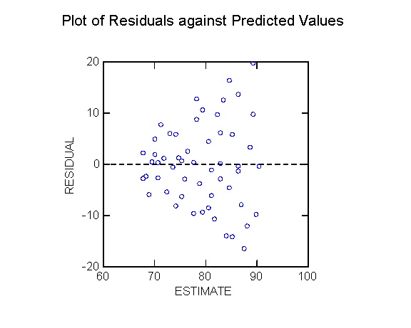
Heteroscedasticity refers to unequal variances
of the error ei
for different observations. It may be visually revealed by a "funnel
shape" in the plot of the residuals ei against the estimates
^Yi or against one of the independent variables Xk.
Effects of heteroscedasticity are the following
-
heteroscedasticity does not bias OLS coefficient
estimates
-
heteroscedasticity means that OLS standard errors
of the estimates are incorrect (often underestimated); therefore statistical
inference is invalid
-
heteroscedasticity means that OLS is not the best
( = most efficient, minimum variance) estimator of b
2. FORMAL DIAGNOSTIC TESTS FOR HETEROSCEDASTICITY
There are many diagnostic tests for heteroscedasticity.
Tests vary with respect to the statistical assumptions required and their
sensitivity to departure from these assumptions (robustness).
1. (Optional) Brown-Forsythe Test
Properties
This test is robust against even serious departures
from normality of the errors.
Principle
Find out whether the error variance
si2
increases or decreases with values of an independent variable Xk
(or with values of the estimates ^Y) by the following procedure:
-
split the observations into 2 groups: one group
with low values of Xk (or low values of ^Y) and another group
with high values of Xk (or high values of ^Y)
-
calculate the median value of the residuals within
each group, and the absolute deviations of the residuals from their group
median
-
then do a t-test of the difference in the means
of these absolute deviations between the two groups; the test statistic
is distributed as t with (n-2) df where n is the total number of cases
An example is shown at the following link:
Exhibit: brown-Forsythe
test with the Afifi & Clark depression data
2. Breusch-Pagan aka Cook-Weisberg
Test
Properties
This is a large sample test; it assumes normality
of errors; it assumes si2
is a specific function of one or several Xk.
Principle
Compare the SSR from regressing ei2
on the Xk to SSE from regressing of Y on the Xk,
with each SS divided by its df; resulting ratio is distributed as c2
with p-1 df.
This is a large-sample test that assumes that
the logarithm of the variance s2
of the error term ei is a linear function of X.
The B-P test statistic is the quantity
c2BP
= (SSR*/(p-1) / (SSE/n)2
where
SSR* is the regression sum of squares
of the regression of e2 on the Xk
SSE is the error sum of squares of the regression
of Y on the Xk
When n is sufficiently large and s2
is constant, c2BP
is distributed as a chi-square distribution with 1 df. Large values
of c2BP
lead to the conclusion that s2
is not constant.
B-P Test in STATA
STATA calls it the Cook-Weisberg test. The
test is obtained with the option hettest used after regress.
The STATA manual states
hettest [varlist] performs 2
flavors of the Cook and Weisberg (1983) test for heteroscedasticity.
This test amounts to testing t=0 in Var(e) = s2exp(zt).
If varlist is not specified, the fitted values are used for z.
If varlist is specified, the variables specified are used for z.
References
This test was developed independently by Breusch
and Pagan (1979) and Cook and Weisberg (1983).
-
Cook, R. D. and S. Weisberg. 1983.
"Diagnostics for Heteroscedasticity in Regression." Biometrika
70:1-10.
-
Breusch, T. S. and A. R. Pagan. 1979.
"A Simple Test for Heteroscedasticity and Random Coefficient Variation."
Econometrica
47:1287-1294.
3. (Optional) Goldfeld-Quandt Test
Properties
Test does not assume a large sample.
Principle
Sort cases with respect to variable believed related
to residual variance; omit about 20% middle cases; run separate regressions
in the low group (obtain SSElow) and high group (obtain SSEhigh);
test F-distributed ratio SSEhigh/SSElow with
(N-d-2p)/2 df in both the numerator and the denominator (where N is the
total number of cases, d is the number of omitted cases, and p is the total
number of independent variables including the constant term).
Reference
-
Wilkinson, Blank, and Gruber (1996:274-277).
3. REMEDIAL APPROACH I: TRANSFORMING Y
If heteroscedasticity is found the first strategy
is to try finding a transformation of Y that stabilizes the error variance.
One can try various transformations along the ladder of powers or estimate
the optimal transformation using the Box-Cox procedure. One variant
of the Box-Cox procedure automatically finds the optimal transformation
of Y given a multiple regression model with p independent variables.
(See STATA reference [R] boxcox. Note that transforming Y
can change the regression relationship with the independent variables Xk.
4. (Optional) REMEDIAL APPROACH II: WEIGHTED
LEAST SQUARES (WLS)
Weighted least squares is an alternative to finding
a transformation that stabilizes Y. However WLS has drawbacks (explained
at the end of this section). Because of this the robust standard
errors approach explaine in Section 5 below has become more popular.
1. Principle of WLS
Unequal error variance implies that the variance-covariance
matrix of the errors ei,
s2{e}
=
| s12 |
0 |
... |
0 |
| 0 |
s22 |
... |
0 |
| ... |
... |
... |
... |
| 0 |
0 |
... |
sn2 |
is such that the variance si2
of ei
may be different for each observation. Errors are still assumed uncorrelated
across observations. Hence the off-diagonal entries of s2{e}
are zeroes and the matrix is diagonal.
Assume (for sake of argument) that the si2
are known.
Then the weighted least squares (WLS) criterion
is to minimize
Qw = Si=1
to n wi(Yi - b0
- b1Xi1
- ... - bp-1Xi,p-1)2
where the weights wi=1/si2
are inversely proportional to the si2;
thus WLS gives less weight to observations with large error variance,
and vice-versa.
2. WLS in Practice
1. Estimating the si2
In practice the si2
(and the weights wi) are not known and must be estimated.
The general strategy for estimating the si2
(and wi) is
-
estimate the regression of Y on the Xk
with OLS and obtain the residuals ei; then
-
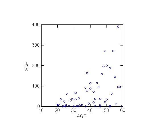
ei2 is an estimator of si2
-
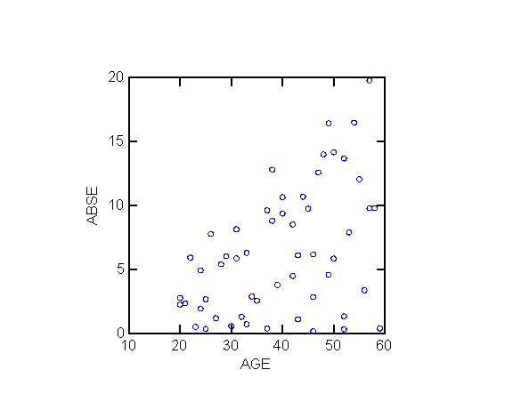
|ei| (the absolute value of ei)
is an estimator of si
-
on the basis of visual evidence (residual plots),
regress either ei2 (to estimate the variance function)
or |ei| (to estimate the standard deviation function)
on
-
one Xk, or
-
several Xk, or
-
^Y (from the OLS regression), or
-
a polynomial function of any of the above
-
the fitted value (estimate) from the regression
is an estimate
-
^vi of the variance si2
(if dependent variable is ei2 ), or
-
^si of the standard deviation si
(if dependent variable is |ei|)
-
calculate the weights wi as either
-
wi = 1/(^si)2
(if ^si was estimated), or
-
wi = 1/^vi (if ^vi
was estimated)
2. Estimating the WLS Regression
Having estimated the wi, the WLS regression
can be done either
-
using a WLS-capable program, by simply providing
the program with a variable containing the weights, say w; the program
automatically minimizes Qw; for example, in SYSTAT enter the
command weight=w prior to the regression
-
using OLS, by multiplying each variable (both
dependent and independent, including the constant) by the square root
of the wi corresponding to a given observation and running
an OLS regression without a constant with the transformed data
These steps can be iterated more than once until
the estimates converge (= Iteratively Reweighted Least Squares - IRLS).
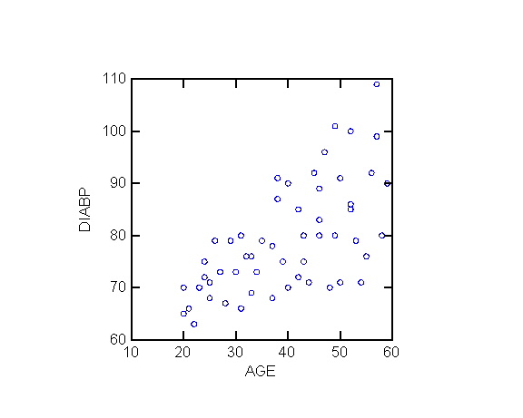
3. Examples of WLS Estimation
Example 1
The following exhibits replicate the analysis
of blood pressure as function of age in ALSM5e pp. <>; ALSM4e pp. <406-407>.
Example 2
The following exhibit carries out a WLS analysis
of the depression model with the Afifi & Clark data.
3. Weighted Least Squares (WLS) as Generalized
Least Squares (GLS)
In this section we show that WLS is a special
case of a more general approach called Generalized Least Squares (GLS).
1. Matrix Representation of WLS
Assume the variance-covariance matrix of e,
s2{e}
as above, with diagonal elements si2
and zeros elsewhere.
The matrix W of weights wi = 1/si2
is defined as W =
| w1 |
0 |
... |
0 |
| 0 |
w2 |
... |
0 |
| ... |
... |
... |
... |
| 0 |
0 |
... |
wn |
Then the WLS estimator of b,
bW
is given by
(X'WX)bW
= X'WY (normal equations)
bW = (X'WX)-1X'WY
Likewise one can show that
s2{bW}
= s2(X'WX)-1
s2{bW}
= MSEW(X'WX)-1
MSEW = Swi(Yi
- ^Yi)2/(n - p)
The WLS estimates can also be obtained by applying
OLS to the data transformed by the "square root" W1/2
of W, where W1/2 contains the square roots of
the wi on the diagonal, and zeros elsewhere.
Since W1/2 is symmetric
and W1/2W1/2 = W, it follows
that
((W1/2X)'(W1/2X))-1(W1/2X)'(W1/2Y)
= (X'W1/2W1/2X)-1(X'W1/2W1/2Y)
= (X'WX)-1(X'WY)
= bW
Thus one can obtain bW
by multiplying Y and X by the square root of the weight and
applying OLS to the transformed data.
2. WLS is a Special Case of Generalized
Least Squares (GLS)
The standard regression model Y = Xb
+ e assumes
that the variance-covariance matrix of the ei
is scalar, that is E{ee'}
= s2I.
Then the OLS estimator
b = (X'X)-1X'Y
has variance matrix
s2{b}
= E{bb'} = E{(X'X)-1X'YY'X(X'X)-1}
s2{b}
= (X'X)-1X'E{YY'}X(X'X)-1
s2{b}
= (X'X)-1X'E{ee'}X(X'X)-1
When the error variance is the same for all observations (homoscedasticity)
then the well-known result for OLS follows:
s2{b}
= (X'X)-1X's2IX(X'X)-1
(because E{ee'}
= s2I)
s2{b}
= s2(X'X)-1X'X(X'X)-1
s2{b}
= s2(X'X)-1
(after cancellation)
And the covariance matrix of errors is estimated
as before as
s2{b}
= MSE(X'X)-1 (estimating s2
as MSE)
and the OLS estimator b is the BLUE of
b
by the Gauss-Markov theorem.
When E{ee'}
is not scalar, it must be represented as E{ee'}
= W where
W
is a (positive definite) symmetric matrix. Then OLS is no longer
the BLUE of b.
Instead, Aitken's (or Generalized Least Squares) theorem states that the
BLUE of b
is
bGLS = (X'W-1X)-1X'W-1Y
where bGLS is termed the generalized
least squares (GLS) estimator.
The matrix W
is usually unknown. When it is possible to estimate W
from the data, the resulting estimator is
bEGLS = (X'^W-1X)-1X'^W-1Y
where ^W
denotes the estimated matrix W.
bEGLS
is termed the estimated generalized least squares (EGLS) or feasible
generalized least squares (FGLS) estimator.
It may be possible to derive a "square root"
of ^W-1,
i.e. a symmetric matrix ^W-1/2
such that (^W-1/2)(^W-1/2)
= ^W-1.
Then an alternative procedure for EGLS estimation is to premultiply X
and Y by ^W-1/2
and use OLS with the transformed data.
In practice, GLS (or EGLS/FGLS) is used when
one has an a priori hypothesis concerning the structure of W.
For example
-
in the heteroscedasticity case one assumes that
W
is a diagonal matrix with elements si2
repressenting the error variance for observation i. Then one only
has to estimate the n error variances si2
to estimate W.
One can see that WLS is a special case of EGLS, with ^W-1
= W.
-
in regression models for time series data with
a first order autoregressive error structure the entries of the W
matrix decrease exponentially away from the diagonal (see Module 14).
On the basis of this systematic pattern one can estimate the matrix W
and estimate b
by EGLS.
-
in regression models for panel data in which one
has t observations over time on n individual units, one assumes that the
error terms contains components that are specific to each unit and/or each
time period. Then W
has a distinctive block-diagonal structure that can be reconstructed by
estimating a small number of parameters. Again one can estimate W
and estimate b
by EGLS.
4. Recommendations on WLS
The WLS approach to heteroscedasticity has at
least two drawbacks.
-
WLS usually necessitates strong assumptions about
the nature of the error variance, e.g. that it is a function of particular
X variable or of ^Y. Sometimes the assumption appears reasonable
(e.g., error variance is proportional to population size, when the units
are areal units); other times it is not.
-
WLS produces an alternative unbiased estimate
of b;
but the OLS estimate is also unbiased. When bOLS
and bWLS differ, which one should one choose?
Today researchers tend to prefer the robust standard
errors approach to heteroscedasticity explained next.
5. REMEDIAL APPROACH III: ROBUST STANDARD
ERRORS
The following discussion relies heavily on Long
and Ervin (2000).
1. Principle of Robust Standard Errors
When heteroscedasticity is present transforming
the variables or the use of WLS may be undesirable when
-
a transformation of the variables that stabilizes
the variances cannot be found
-
a suitable transformation is found, but the resulting
non-linear model is difficult to interpret substantively
-
the weights to use in WLS cannot be found, as
when the functional form of the heteroscedasticity is not known
The alternative strategy can be used even when
the form of the heteroscedasticity is unknown. It consists of
-
estimating b using OLS as usual
-
use a heteroscedasticity consistent covariance
matrix (HCCM) to estimate the standard errors of the estimates; these
standard errors are then called robust standard errors
There are 3 variants of the strategy, labelled
HC1, HC2, and HC3. To explain the principle of HCCM start with the
usual multiple regression model
Y = Xb
+ e
where E{e}
= 0 and E{ee'}
= W is
a positive definite matrix.
Then the covariance matrix of the OLS estimate
b
= (X'X)-1X'Y is
s2{b}
= (X'X)-1X'WX(X'X)-1
When the errors are homoscedastic, W
= s2I
and the expression for s2{b}
reduces to the usual
s2{b}
= s2(X'X)-1
OLSCM = s2{b} = MSE(X'X)-1
(where MSE = Sei2/(n-p))
OLSCM denotes the usual OLS covariance matrix
of estimates.
2. Huber-White Robust Standard Errors HC1
The basic idea of robust standard errors is that
when the errors are heteroscedastic one can estimate the observation-specific
variance si2
with the single observation on the residual as
^Wii
= (ei - 0)2/1 = ei2
^W
= diag{ei2}
This leads to the HCCM
HC1 = (n/(n-p)) (X'X)-1X'diag{ei2}X(X'X)-1
where n/(n-p) is a degree of freedom correction
factor that becomes negligible for large samples.
HC1 is called the Huber-White estimator (after
Huber 1967; White 1980) or the "sandwich" estimator because of the appearance
of the formula. (See it?)
HC1 is obtained in STATA using the robust option (e.g., regress
y x1 x2, robust).
3. HC2
An alternative to HC1 proposed by MacKinnon and White (1985) is to use
a better estimate of the variance of ei
based on s2{ei}
=
s2(1
- hii) where hii represent the leverage of observation
i (diagonal element of the hat matrix H); the alternative formula divides
the squared residual by (1 - hii)
HC2 = (X'X)-1X'diag{ei2/(1
- hii)}X(X'X)-1
HC2 is obtained in STATA using the hc2 option (e.g., regress
y x1 x2, hc2).
4. HC3
A third possibility has a less straightforward theoretical motivation (Long
and Ervin 2000; although compare the formula for HC3 with that for the
deleted residual di in Module 10). The idea is to "overcorrect"
for high variance residuals by dividing the squared residual by (1 - hii)2.
This yields
HC3 = (X'X)-1X'diag{ei2/(1
- hii)2}X(X'X)-1
HC3 is obtained in STATA using the hc3 option (e.g., regress
y x1 x2, hc3).
5. Relative Performance of HC1, HC2 and HC3 Robust Variance Estimators
Long and Erwin (2000) conclude from an extensive series of computer simulations
that the HC3 gives the best results overall in small samples in the presence
of heteroscedasticity of various forms. They state
"1. If there is an a priori reason to suspect that there
is heteroscedasticity, HCCM-based tests should be used."
"2. For samples less than 250, HC3 should be used; when samples
are 500 or larger, other versions of the HCCM can also be used. The
superiority of HC3 over HC2 lies in its better properties when testing
coefficients that are most strongly affected by heteroscedasticity."
"3. The decision to correct for heteroscedasticity should not
be based on the results of a screening test for heteroscedasticity."
"Given the relative costs of correcting for heteroscedasticity using HC3
when there is homoscedasticity and using OLSCM tests when there is heteroscedasticity,
we recommend that HC3-based tests should be used routinely for testing
individual coefficients in the linear regression model."
6. Example of Robust Standard Errors Estimation
The following exhibit shows the use of the HC1 (robust), HC2 (hc2)
and HC3 (hc3) robust standard errors with STATA
6. CONCLUSION: DEALING WITH HETEROSCEDASTICITY
Provisional guidelines for dealing with the possibility
of heteroscedasticity are
-
look at the plot of OLS residuals against estimates;
if there is a suggestion of a funnel shape use a test of heteroscedasticity;
use the Breusch-Pagan a.k.a. Cook-Weisberg test as it is easy to do in
STATA; use one of the other tests (modified Levene or Goldfeld-Quandt)
if you have a reason to, such as a small sample or doubts about normality
of errors
-
if there is heteroscedasticity look first for
a reasonable transformation that might stabilize the variances of the errors,
but without introducing problems of interpretation or upsetting the functional
relationship of Y with the independent variables; if such a transformation
is found it is a desirable solution
-
if a suitable transformation cannot be found,
investigate the possibility of WLS; try estimating the variance function
or the standard deviation function; if a convincing function is found (one
that has substantial R2 and/or one that makes substantive sense,
such as when the error variance is proportional to some measure of the
size of the unit) then try WLS; otherwise, use the robust standard error
approach instead (next)
-
if the transformation approach and the WLS approach
do not seem promising, then use the robust standard errors approach; follow
the recommendations of Long and Ervin (2000) to choose between HC1, HC2
and HC3, at least until someone comes up with evidence to the contrary;
alternatively, adopt this approach right away after failing to find a good
variance-stabilizing transformation, bypassing WLS
Last modified 17 Apr 2006