Soci709 (formerly 209) Module 10 - OUTLYING &
INFLUENTIAL OBSERVATIONS
1. ADDED-VARIABLE PLOTS FOR FUNCTIONAL FORM
& OUTLYING OBSERVATIONS
1. Uses of Added-Variable Plots
Added-variables plots are also called partial
regression plots and adjusted variable plots.
A partial regression plots is a diagnostic
tool that permits evaluation of the marginal role of an individual variable
within the multiple regression model, given that other independent variables
are in the model. The plot is used to visually assess
-
whether a variable has a significant marginal
association with Y (given other independent variables already in model)
and thus should be included in the model
-
the presence of outliers and influential cases
that affect the coefficients of an individual X variable in the model
-
the possibility of a nonlinear relationship between
Y and individual X variable in the model
An added-variable plot is a way to look at the
marginal role of a variable Xk in the model, given that the
other independent variables are already in the model.
2. Construction of an Added-Variable Plot
Assume the multiple regression model (omitting
the i subscript)
y = b0
+ b1X1
+ b2X2
+
b3X3
+ e
There is an added-variable plot for each one of
the X variables.
To draw the added-variable plot of y on X1
"the hard way", for example, one proceeds as follows:
1. Regress y on X2 and X3
and a constant, and calculate the predictors (denoted ^yi(X2,
X3) and residuals (denoted ei(y|X2, X3)
for y regression
^yi(X2, X3)
= b0 + b2Xi2 + b3Xi3
ei(y|X2, X3)
= yi - ^yi(X2, X3)
2. Regress X1 on X2
and X3 and a constant, and calculate the predictors and residuals
for X1
^Xi1(X2, X3)
= b0+ + b2+Xi2 +
b3+Xi3
ei(X1|X2,
X3) = Xi1 - ^Xi1(X2, X3)
3. The added-variable plot for X1
is the plot of
ei(Y|X2, X3)
against ei(X1|X2, X3)
In words, the added-variable plot for a given
independent variable is the plot of the residuals of y (regressed on the
other independent variables in the model plus a constant) against the residuals
of the given independent variable (regressed on the other independent variables
in the model plus a constant). In practice, statistical programs such as
STATA and SYSTAT have options to produce these plots automatically without
the need for auxilliary regressions.
3. Interpretation of an Added-variable Plot
& Example
It can be shown that the slope of the partial
regression of ei(y|X2, X3) on ei(X1|X2,
X3) is equal to the estimated regression coefficient b1
of X1 in the multiple regression model y = b0
+ b1X1
+ b2X2
+
b3X3
+ e .
Thus the added-variable plot allows one to isolate the role of the specific
independent variable in the multiple rgeression model. In practice
one scrutinizes the plot for patterns such as the ones shown in the next
exhibit.
The patterns mean
-
pattern (a), which shows no apparent relationship,
suggests that X1 does not add to the explanatory power of the
model, when X2 and X3 are already included
-
pattern (b) suggests that a linear relationship
between y and X1 exists, when X2 and X3
are already present in the model; this suggests that X1 should
be added to (or kept in)
-
pattern (c) suggests that the partial relationship
of y with X1 is curvilinear; one may try to model this curvilinearity
with a transformation of X1 or with a polynomial function of
X1
-
the plot may also reveals observations that are
outlying with respect to the partial relationship of y with X1
Example. In the graduation rates study units
are U.S. states plus Washington DC. The dependent variable (GRAD)
is the rate of graduation from high school. The following model is
estimated
GRAD = CONSTANT + INC + PBLA + PHIS
+ EDEXP + URB.
Data and regression results are shown in the next
2 exhibits.
SYSTAT Plots
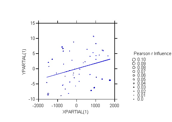
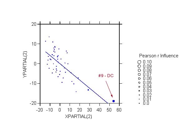
The added-variable plots for INC, PBLA, and PHIS
are
As an extra refinement the SYSTAT plots use the
INFLUENCE option. In an influence plot the size of the symbol is
proportional to the amount that the Pearson correlation between Y and X
would change if that point were deleted. Large symbols therefore
corespond to observations that are influential. The plots allow us
to identify cases that are problematic with respect to specific independent
variables in the model. For example, two observations stand out:
DC in the plot for PBLA, and NM in the plot for PHIS.
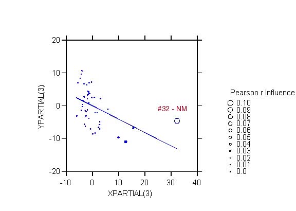
The style of the symbol indicates the direction
of the influence:
-
an open symbol indicates an observation
that decreases (i.e., whose removal would increase) the magnitude
(absolute value) of the bivariate correlation; for example, removing NM
(case 32) in the added-variable plot for PHIS would increase the magnitude
of the correlation between residual of y and residual of PHIS from -.461
to -.558.
-
a filled symbol indicates an observation
that increases (i.e., whose removal would decrease) the magnitude
(absolute value) of the correlation; for example, removing DC (case 9)
in the partial regression plot for PBLA would decrease the magnitude of
the correlation between residual of y and residual of PBLA from -.703 to
-.641.
As I was not sure of the statistic used to determine
the size of symbols with the INFLUENCE option I sent questions to the SYSTAT
users list, which were answered by SYSTAT's founder Leland Wilkinson.
It turns out that SYSTAT calculates the influence of an observation very
simply as the absolute value of the difference in the correlation coefficient
of Y and X with and without that observation.
The added-variable plot can also suggest that
the marginal relationship between y and an independent variable is non-linear.
Nonlinearity could be visualized using a lowess nonparametric regression.
For example one might use lowess to verify that teh added-variable plot
for PBLA is linear.
STATA Plots
The following link shows the same plots produced by STATA.
2. THREE TYPES OF OUTLYING OBSERVATIONS
-
an outlying case is one with an observation
that is well separated from the remainder of the data
-
an influential case is one that has a substantial
influence on the fitted regression function (i.e., the estimated regression
function is substantially different depending on whether the case is included
or not in the data set)
A case can be outlying with respect to their Y
value or X value(s) and an outlying case may or may not be influential.
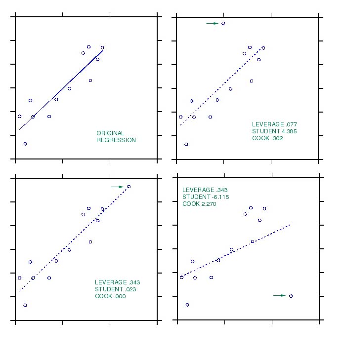
This is shown with an artificial data set by adding cases with different
kinds of outlyingness:
In these plots
-
Case #1 is outlying with respect to its Y value,
but not influential. (Why?)
-
Case #2 is outlying with respect to its X value,
but not influential. (Why?)
-
Case #3 and #4 are outlying with respect to both
Y
and X values, and are influential. (Why?)
Diagnostic tests have been developed to identify
three
types of problematic observations:
-
observations outlying in the X-dimensions, called
high
leverage observations
-
observations outlying in the Y-dimension
-
influential observations
3. IDENTIFYING X-OUTLYING OBSERVATIONS -
LEVERAGE
In multiple regression X-outlying observations
are identified using the hat matrix H.
1. Review of the Hat Matrix
We saw in Module 4 that the nx1 vector ^y
of estimated (predicted, fitted) values of y is obtained as
^Y = HY
where
H = X(X'X)-1X')
One can view the nxn matrix H as the linear
transformation that transforms the observations y on the dependent
variable into their estimated values ^y in terms of X.
The vector of residuals e can also
be expressed in terms of H as
e = (I - H)y
(collecting terms)
Both H and (I - H) are symmetric
and idempotent, so that
H' = H and HH = H
(I - H)' = (I - H) and (I
- H)(I - H) = (I - H)
Q - How can one show that H and (I
- H) are symmetric and idempotent?
It follows that the variance-covariance matrix
of the residuals e, both "true" and estimated are
s2{e}
= E{[(I - H)y][(I - H)y]'} = s2(I
- H)
s2{e}
= MSE(I - H) (where MSE is the estimate of the variance s2
of e)
Note: These formulas follow from the fact that if
A is a linear
transformation and y a random vector then
s2{Ay}
= As2{y}A'
In this case e = (I - H)Y,
therefore
s2{e}
= s2{(I-H)Y}
= (I-H)s2I(I-H)'
= s2(I-H)(I-H)
= s2(I-H)
using the fact that I-H is symmetric and
idempotent. |
Thus the variance of an individual residual
ei (i.e., the diagonal element of the variance-covariance
matrix s2{e} corresponding
to observation i) is
s2{ei}
= s2(1
- hii)
s2{ei} = MSE(1 - hii)
where hii denotes the ith element on
the main diagonal of H.
hii is called the leverage
of observation i.
hii can be calculated without calculating
the whole H as
hii = xi'(X'X)-1xi
where xi' is the row
of X corresponding to observations on case i. Thus xi'
= [1 Xi1 Xi2 ... Xi,p-1]
(and
xi is the same thing transposed as a column
in
X'.)
Q - What is the dimension of hii
. What kind of expression is xi'(X'X)-1xi
? (Hint: It is a q... f...)
It can be shown that
0 <= hii <= 1
Si=1 to n
hii = p
Q - Why is the sum of the hii equal
to p? See next box (optional).
Geometric Glimpse (Optional)
H is an idempotent matrix and thus a projection
H projects a point y in n-dimensional
space onto a point ^y that lies in the p-dimensional subspace spanned
by the p columns of X
the trace of an idempotent matrix, which
is the sum of the diagonal elements, is equal to the dimension of the
subspace onto which points are projected
that is why the sum of the hii (i.e.,
the trace of H) is p
|
2. hii Measures the Leverage
of an Observation
A larger value of hii indicates that
a case has greater leverage in determining its own fitted value
^Yi . This can be seen in 2 ways:
-
in the formula ^y = Hy hii
represents the weight of observation Yi in calculating its
own fitted value ^Yi
-
since s2{ei}
= s2(1
- hii) it follows that the larger hii, the smaller
s2{ei},
and the closer ^yi will be to yi. (At the limit,
if hii =1, ^yi is forced to be equal to yi,
which means that observation i has so much leverage that it "forces" the
regression plane to go through itself.)
More on the meaning of hii:
hii is related to the distance
between
xi and X. , which
is the vector of the sample means of the X variables, called the centroid
of
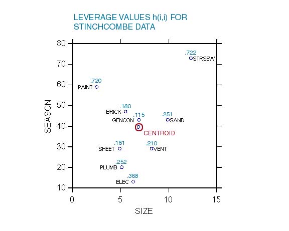
X. This property is illustrated by calculating H
for the construction industry data.
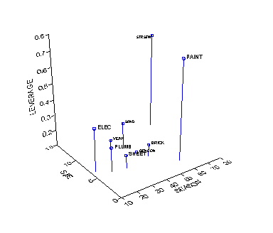
Plotting observations in the SIZE x SEASON space
(shown as a 2-D or 3-D plot) shows that observations distant from the centroid
have larger leverage.
3. Using the Leverage hii for
Diagnosis
We look at leverage for the graduation rate data.
There are 3 ways of identifying high-leverage
observations:
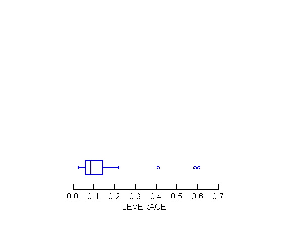
-
look at a box plot or stem-and-leaf plot of hii
for (an) extreme value(s) of hii
-
rule of thumb #1: consider hii large
if it is larger than twice the average hii. Since the
sum of hii (trace of H) is p (=number of independent
variables including the constant term), average hii is p/n.
Thus flag observations for which hii > 2p/n
-
rule of thumb #2: take hii > 0.5 to
indicate "VERY HIGH" leverage; 0.2 < hii < 0.5 to indicate
"MODERATE HIGH" leverage.
In the graduation rate example:
-
the stem & leaf plot of leverage flags AK,
DC, and NM as "outside values"
-
since n=51 and p=6, 2p/n = .235; this criterion
is exceeded by AK (.409), DC (.587), and NM (.605)
-
DC and NM also exceed the hii > 0.5
criterion and are thus considered VERY HIGH leverage; AK is considered
MODERATE HIGH.
Looking back at the original data often reveals
why an observation is outlying in the X-space. (Why would AK, DC
and NM be X-outliers?)
4. Identifying Hidden Extrapolation
An important point about leverage is that it depends
only on the X matrix, not the value of y. Thus one can calculate
the leverage for a new combination xnew of values not found
in the data set. This allows identifying hidden extrapolation.
See ALSM5e p. 400 for details.
4. IDENTIFYING Y-OUTLYING OBSERVATIONS aka
THE QUEST FOR THE ULTIMATE RESIDUAL
Efforts to find the best diagnostic test for outliers
in the Y dimension have produced successive improvements to the ordinary
residual ei calculated as
ei = Yi - ^Yi
or, in matrix notation,
e = Y - ^Y
1. Standardized (aka Semi-Studentized) Residual
ei*
The first improvement is the standardized residual,
calculated by dividing the raw residual by the estimated standard deviation
of the residuals s=MSE1/2 as
ei* = ei/(MSE)1/2
This is simply the residual ei divided
by the square root of MSE. Since the mean of teh residuals is zero,
ei* is equivalent to a z-score.
2. (Internal) Studentized Residual ri
The internal studentized residual ri
is the ratio of ei to a more precise estimate of the standard
deviation of ei, s{ei} = (MSE(1
- hii))1/2 so that
ri = ei/s{ei}
= ei/(MSE(1 - hii))1/2
This refinement takes into account that the residual
variance varies over observations. (From the formula s2{e}
= MSE(I - H).)
3. External or Deleted Residual di
The problem with the internal studentized residual
is that ei = yi - ^yi may be artificially
small if case i has high leverage which forces ^yi to be close
to yi (thereby reducing the variance of ei).
To avoid this one estimates the residual for case i based on a regression
that excludes (i.e., "deletes") case i . This is the deleted
residual defined as
di = yi - ^yi(i)
where the notation ^yi(i) means the
fitted value of y for case i using a regression with (n-1) cases excluding
(or "deleting") case i itself. (This is why di is also
called external, because case i is not involved in the regression
producing the residual.) It sounds like to calculate di
one has to run n regression, one for each case. In fact an
equivalent formula for di that only involves the regression
with the n cases is
di = ei/(1 -
hii)
4. Studentized External Residual or Studentized
Deleted Residual ti
Since di = ei/(1 - hii)
its variance is estimated as
s2{di} = MSE(i)/(1
- hii)
and its standard deviation as
s{di} = [MSE(i)/(1
- hii)]1/2
The last improvement is obtained by dividing
di by its standard deviation. The studentized deleted
residual ti is obtained as
ti = di/s{di}
or, equivalently (ALSM5e pp. 396; ALSM4e pp. 373-374)
as
ti = ei((n -
p - 1)/(SSE(1 - hii) - ei2))1/2
which only involves the regression with the n
cases.
What is the distribution of ti?
A useful observation is that ^yi(i) is the same thing as ^yh(new)
discussed earlier. ^yi(i) is calculated from a regression
with n-1 cases (excluding case i) while ^yh(new) is calculated
for a new set of X values from an original regression based on n cases.
It follows from the similarity with yh(new) that
ti = di/s{di}
~ t(n - p - 1)
In words, ti is distributed as a Student
t distribution with (n-p-1) df. (The df are (n-p-1) rather than (n-p)
because there are n-1 cases left after case i has been deleted.)
Using ti in Testing for y-outliers
Knowing that
ti = di/s{di}
~ t(n - p - 1).
one can test whether a residual is larger than
would be expected by chance. But one cannot just test at the a
= .05 level by looking for absolute values of ti greater than
about 2, because there are n residuals and thus de facto n tests.
One approach to multiple tests is to use the Bonferroni criterion which
divides the original a
by the number n of tests. The Bonferroni-corrected critical value
to flag ouliers is thus
t(1 - a/2n;
n - p - 1)
Cases with values of the studentized deleted residual
ti greater in absolute value than this critical value are flagged
as outliers.
Graduation Rate Example
SYSTAT saves the studentized deleted residuals
ti under the name STUDENT. Choose a
= .05. Since n = 51 and p = 6, the critical value is t(1-0.05/102;
44) = t(0.99951; 44). Using the SYSTAT calculator
>calc tif(0.99951, 44)
3.532676
The largest value of STUDENT is 2.840 (NM).
But that's not large enough for NM to be considered an outlier, according
to the Bonferroni criterion! So we would conclude that none of the
observations is an outlier, using the Bonferroni approach. Clearly
this is not very satisfactory, and an alternative to the Bonferroni criterion
is needed.
NOTE: The Bonferroni criterion is very conservative,
so the development of alternative ways of testing residuals for outliers
is an active field of research. An article by Williams, Jones, and
Tukey (1999) provides an alternative to the Bonferroni criterion that ends
up flagging more cases as outliers.
The important point is that it may not be necessary
to rigorously test whether a case is an outlier, since the degree to which
an outlier is problematic depends on whether it is influential. Thus
one would not take action solely on the basis of a significant Studentized
deleted residual.
5. IDENTIFYING INFLUENTIAL CASES - DFFITS,
COOK, and DFBETAS
A case is influential if excluding it from
the regression causes a substantial change in the estimated regression
function. There are several measures of influence: DFFITS, COOK (Cook's
distance), and DFBETAS. Personally I prefer to use the Cook distance
for reasons explained below.
1. DFFITS
DFFITS measures the influence that case i has
on its own fitted value ^yi as
DFFITSi = (^yi
- ^yi(i))/(MSE(i)hii)1/2
In words, DFFITSi represents the difference
in predicted values of yi from regressions with (^yi)
or without (^yi(i)) case i, the difference being expressed
in units of the standard deviation of the predicted yi (in which
MSE is estimated from the regression without case i). Thus it is
a standardized measure of the extent to which incluion of case i in the
regression increases or decreases it own predicted value. DFFITSi
can be positive or negative.
An equivalent formula that only involves the
regression with the n cases is
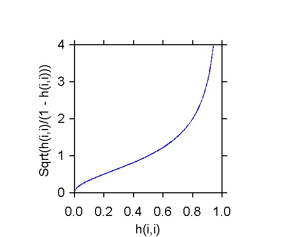
DFFITSi = ti(hii/(1
- hii))1/2
The formula shows that DFFITSi is the
product of the studentized deleted residual ti multiplied by
a function ot the leverage hii. Thus DFFITSi
tends to be large when a case is both a Y-outlier (large ti)
and
has large leverage (large hii). The effect of the
factor (hii/(1 - hii))1/2 is shown in
the next exhibit.
Using DFFITS in Identifying Influential Cases
(ALSM5e p. 401; ALSM4e p. 379) offer the following
guidelines for identifying influential cases
-
|DFFITS| > 1 (small to medium data sets)
-
|DFFITS| > 2(p/n)1/2 (large data sets)
Graduation Rate Example
SYSTAT does not automatically calculates DFFITS
so I computed DFFITS with the statement
>let dffits = student*sqr(leverage/(1-leverage))
In the graduation rate data n=51 and p=6 so that
2(p/n)1/2 = 2(6/51)1/2 = .686.
Looking down the column with the values of
DFFITS for values greater than .686 one finds
-1.876 (#2 AK)
1.260 (#9 DC)
3.514 (#32 NM)
These cases are thus considered to be influential
according to the guidelines.
2. COOK's Distance Di
COOK's distance measures the influence of case
i on all n fitted values ^yi (not just the fitted value
for case i as DFFITS). Di is defined as
Di = (^y - ^y(i))'(^y
- ^y(i)) / pMSE
where the numerator is the sum of the squared
differences between the fitted values of y for regressions with case i
included or excluded, respectively. It can be shown that an equivalent
formula that only involves the regression with the n cases is
Di = (ei2/pMSE)(hii/(1
- hii)2)
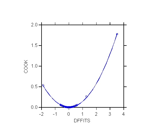
The formula shows that Di is large
when either the residual ei is large, or the leverage hii
is large, or both. In practice, one finds that Di is almost
a quadratic function of DFFITS. As Di is (approximately)
proportional to squared DFFITS it tends to amplify the distinctiveness
of influential cases, making them stand out.
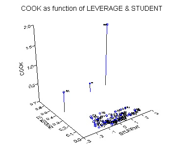
Another way to look at the way COOK measures a
combination of high leverage (large value of hii) and a large
residual is to look at a plot of COOK against LEVERAGE and STUDENT.
The plot is obtained in SYSTAT with the command
>plot cook*leverage*student/stick=out
spike label=state$
The figure shows how 3 high-influence cases stand
out in the zone of high leverage. In that zone, influence is greater
when the residual is larger (compare AK and NM with DC, which has a smaller
studentized residual).
Using Di (COOK) in Identifying Influential
Cases
It has been found useful to relate the values
of COOK to the corresponding percentiles of F(p, n-p) distribution.
NKNW (p. 381) offer the following advice: "If the percentile value is...
-
less than about 10 or 20 percent ... the ith case
has little apparent influence...
-
near 50 percent or more ... the ith case has a
major influence..."
(One would like a more definite statement!
What does one do when COOK is between 20 and 50 percent?)
Graduation Rate Example
SYSTAT saves Di under the name COOK.
I calculated the percentiles of the F(p, n - p) = F(6, 51 - 6) distribution
in the last column of the diagnostics with the SYSTAT statement
>let fperc = 100*fcf(cook, 6, 45)
Large values of COOK really stand out
#2 AK 0.538 (%F 22.3)
#9 DC 0.264 (%F 4.9)
#32 NM 1.778 (%F 87.5)
Thus the usual suspects come up with larger COOK
values but DC does not make the "10 or 20" percent cut as an influential
case.
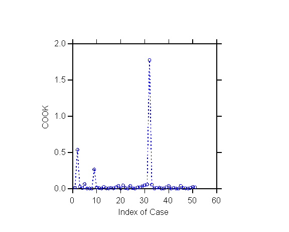
The COOK statistic is perhaps the best summary
indicator of influence, as it tends to amplify the influence of a case
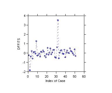
relative to DFFITS. Thus the quickest way to detect influential cases
is to plot COOK against the case number (this is called an index plot)
and flag cases that stand out. I produced such a plot in SYSTATwith
the command
>plot cook/stick line dash=11
Compare this to the index plot of DFFITS.
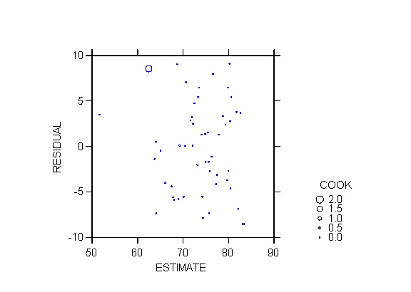
Another useful plot is the proportional influence
plot, in which the residual ei (or any other variant) is
plotted against ^Yi with the size of symbols proportional to
the Cook distance (ALSM5e Figure 10.8 p. 404; ALSM4e Figure 9.8 p. 382).
I produced such a plot in SYSTAT with the command
>plot residual*estimate/stick size=cook
3. DFBETAS
(DFBETAS)k(i) is a measure of the influence
of the ith case on the regression coefficient of Xk. Therefore
there is a DFBETAS for each Xk (k = 0, ..., p-1). The
formula is
(DFBETAS)k(i) = (bk
- bk(i))/(MSE(i)ckk)1/2
for k = 0, 1, ..., p-1
where ckk is the kth diagonal element
of (X'X)-1. (Recall the formula for the variance of bk
, s2{bk}
= s2ckk.).
NKNW's guideline is to flag a case as influential
if
-
DFBETAS > 1 (small to medium data sets)
-
DFBETAS > 2/(n)1/2 (large data sets)
The problem with DFBETAS is that there are p of
them, which is a lot of output, so it is usually easier to look at summary
diagnostic measure such as Di. SYSTAT does not automatically
calculate the DFBETAS and I don't know a formula that is based on the regression
with n cases, although one surely exists. See ALSM5e Table 10.4 p.
402 and pp. 404-405; ALSM4e Table 9.4 p. 380 and pp. 382-383 for an example
of the use of DFBETAS.
4. Influence on Inferences
Once influential cases have been (even tentatively)
identified one can measure their overall influence on the estimated regression
function as the average absolute percent difference in the estimated y
(1/n)Si=1
to n |(^yi(d) - ^yi)/^yi|100
where ^yi(d) denotes the predicted
values of Y from a regression excluding the influential case(s). (The summation
is over all n cases.)
If the average absolute percent difference
is small it may not be necessary to take any action about the influential
cases.
Graduation Rate Example
With all cases included (n=51) the estimated regression
function is
GRAD = 69.042 + .002INC - .414PBLA
- .407PHIS - .001EDEXP - .108URB
With AK, DC and NM excluded (n = 48)
GRAD = 62.613 + .002INC - .452PBLA
- .759PHIS - .001EDEXP - .110URB
The average absolute percent difference is 11.154%,
which seems too large to ignore.
6. SUMMARY OF DIAGNOSTICS FOR OUTLIERS &
INFLUENTIAL CASES
A useful way to study diagnostics is to construct
one's own summary table of guidelines and cutoff points for the diagnostics
that are most often used in practice: leverages hii, studentized
deleted residuals ti, COOK (Di) and/or DFFITS, and
perhaps DFBETAS.
What diagnostics to use for routine work?
(See also Fox 1991, pp. 75-76)
-
keep in mind that influential cases are more common
in small data sets (except for grossly inaccurate coding such as missing
values treated as real data)
-
look at index plot of Cook's Di (or
DFFITS) as a good summary measure of influence; use the test of COOK based
on a comparison with an F distribution to test apparent influential observations
-
look at a stem-and-leaf or box plot of STUDENT
(studentized deleted residual); look especially for the observations flagged
by COOK
-
look at a stem-and-leaf or box plot of LEVERAGE
(hii); look especially for the observations flagged by COOK
-
look at partial regression plots to see how the
"suspects" affect individual regression coefficients
These examinations usually narrow down the search
to a small number of cases and reveal their "personality", i.e. the ways
in which they are "deviant", possibly suggesting already remedial strategies.
In my epxerience it is rarely necessary to look further than this.
7. REMEDIES FOR OUTLIERS & INFLUENTIAL
CASES
1. Get Rid of Them Outliers?
Outlying and influential cases should not be discarded
automatically.
There are several situations:
-
if the case is the result of recording error and
such, then
-
if possible, correct the observation
-
if not, discard it
-
if the case is not clearly erroneous, examine
adequacy of the model; influential/outlying observation could be due
to
-
omission of an important interaction (so that
a case with high values of the two variables involved in the interaction
has an extreme value of Y)
-
incorrect functional form
-
omission of an important explanatory variable;
Example: several outliers are oil-exporting countries; then maybe including
an indicator variable for oil-exporting countries will take care of the
problem
-
discard cases that cannot be accounted for by
above only as last resort, reporting whether results differ with the cases
included or excluded; or use robust estimation method to reduce their influence
(see below)
2. Robust Regression
1. Varieties of Robust Regression Methods
Robust regression methods are less sensitive than
OLS to the presence of influential outliers. There are several approaches
to robust regression such as
-
least absolute residuals (LAR) regression minimizes
the sum of absolute (rather than squared) deviations of Y from the regression
function
-
least median of squares (LMS) regression minimizes
the median (rather than the sum) of squared deviations of Y from the regression
function
-
trimmed regression excludes a certain percentage
of extreme cases at both ends of the distribution of residuals
-
iteratively reweighted least squares (IRLS) iteratively
reweights cases in inverse proportion to its residual (standardized by
the robust estimator of dispersion MAD discussed below) to discount the
influence of extreme cases; IRLS refers to a family of methods distinguished
by different weigthting functions (such as Huber, Hampel, bisquare, etc.)
2. Iteratively Reweighted Least Squares
(IRLS) with MAD Standardized Residual
IRLS methods discount the weight of outlying cases
in the regression as a function of residuals standardized using a robust
estimate of s
called median absolute deviation (MAD)
MAD = (1/.6745) median{|ei
- median{ei}|}
where the term .6745 is a correction factor to
make MAD an unbiased estimate of the standard deviation of residuals from
a normal distribution.
The robust standardized residual ui
for observation i is
ui = ei/MAD
Given ui the cases are weighted according
to a variety of functions.
See NKNW pp. 416-424 for a detailed example of
the process using the Huber function.
The following two exhibits show robust regressions
of the GRAD data using the NONLIN module of SYSTATand a variery of robust
regression approaches.
The following exhibit shows how to do robust regression
in STATA 6 (median regression and combination of Hampel / bisquare methods
only).
3. The Hadi Robust Outlier Detection Method
The new Hadi method of robust outlier detection
has two features differentiating it from classical outlier diagnostics
and remedies (Hadi 1992, 1994; SYSTAT V6.0/V7.0 Statistics pp. 319-322):
-
classical diagnostic tools for outliers and influential
cases are fully justified only for a single outlier/influential case and
the simultaneous presence of several such cases can defeat the diagnostics
(because of the "swamping" and "masking" problems); by contrast, the Hadi
method is effective even in the presence of several outliers/influential
observations
-
the Hadi method does not distinguish between
y-outlying and X-outlying observations as it uses a single matrix (say
Z)
that combines the dependent variable Y and independent variables
X,
so that Z = [Y X]; the method calculates robust estimates
of the distances of the observations Zi from the centroid of
Z
(so it can be used for purposes other than regression analysis) and identifies
as outliers observations that are "too far" from the centroid according
to a certain criterion
The Hadi method is implemented in the CORR module
of SYSTAT that calculates matrices of covariances, correlations, and distances.
To use the Hadi method for multiple regression one can either
-
calculate the matrix of covariances or correlations
in CORR using the Hadi option so that outliers are deleted, and then use
that matrix to run the multiple regression; this strategy is shown in the
exhibit below
-
or calculate any of these matrices in CORR just
for the purpose of identifying outliers; then run the regression in the
usual way after selecting out the outliers
As far as we can figure out at the moment the
Hadi procedure as implemented in SYSTAT consists of the following steps
-
compute a robust covariance matrix by finding
the median for each variable and using deviations from the median in calculating
sums of squares and cross-products (special steps are taken if the resulting
covariance matrix is singular)
-
use this robust matrix to compute the distance
of each case from the centroid (determined by the medians) using the formula
Zi'(Z'Z)-1Zi
(similar to the formula for hii; this is called the Mahalanobis
distance); rank the cases according to distance from the centroid
-
use the half of the data set with the lowest ranks
(i.e., closest to the centroid) to compute the usual covariance matrix
(using deviations from the mean)
-
use this covariance matrix to compute new distances
for all the cases and rerank them
-
select the same number of the cases with smallest
ranks plus one and repeat the process, each time updating the covariance
matrix, computing new distances and reranking the cases, and increasing
the subset of cases by one
-
continue adding cases until the entering one exceeds
a certain chi-square based criterion explained in Hadi (1994); the remaining
cases are identified as outliers
-
use the cases that are not identified as outliers
to computer the covariance matrix in the usual way
For the GRAD data the Hadi procedure identifies
more cases as outliers than the classical diagnostics do.
8. STATA COMMANDS
use "Z:\mydocs\s209\grad.dta", clear
regress grad inc pbla phis edexp urb
* first plot residuals vs. fitted values
rvfplot, yline(0)
* next do a plot of leverage against squared normalized residual
* the STATA manual recommends this plot
lvr2plot
* redo plot with label on the points, so we know what state it is
lvr2plot, mlabel(state)
* next do added-variable plots for all X variables
avplots
* can also request added-variable plot for only one X variable
avplot phis, mlabel(state)
* STATA also has a component-plus-residual plot but I don't understand it
cprplot phis, lowess
* STATA also has an augmented component-plus-residual plot that's supposed ro be
better
* to evaluate functional form
acprplot phis, mlabel(state) lowess
* next calculate leverage, studentized residual, cook's distance, dffits,
dfbetas
* if e(sample) expression used to restict estimates to the sample used in
regression; not needed here
predict lev, leverage
predict stu, rstudent
predict cook, cooksd
predict dfits, dfits
* the dfbeta command generates all the dfbetas in one swoop
dfbeta
* STATA has used the original variable name with DF prefix
* next calculate the percentile of F(p, n-p) distribution of cook
generate Fperc=100*(1 - Ftail(6, 45, cook))
list state lev stu cook Fperc dfits
* another way to see influential cases is an index plot
graph twoway line Fperc id, mlabel(state)
* next do Hadi multivariate outliers analysis
. hadimvo grad inc pbla phis edexp urb, generate(hadiout mahadist) p(.05)
* you should find STATA reports 16 outliers; you can look at them with
* the command
. list state hadiout mahadist
* next redo hadimvo with lower probability of rejection
. hadimvo grad inc pbla phis edexp urb, generate(hadiout2 mahadist2) p(.001)
* how many outliers are there now? who are they? find out with
. list state hadiout2 mahadist2
* next do robust regression; look at the output and try to guess
* why the regression has only 50 observations
.
rreg grad inc pbla phis edexp urb
Last modified 6 Apr 2006